napari-lsft

Light Sheet Fluorescence Tomography — napari plugin for 3D reconstruction from rotational light-sheet microscopy data.

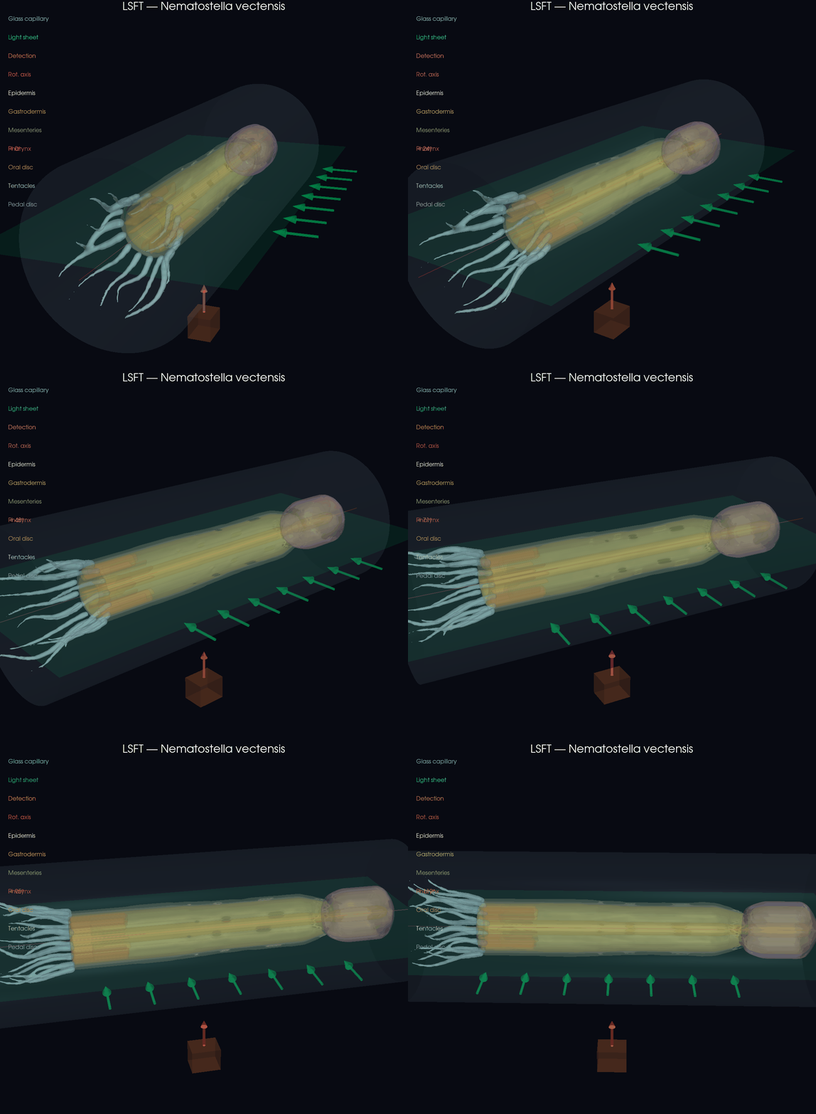
Principle, shown on a Nematostella vectensis phantom: a thin light sheet optically sections the sample inside the capillary while it rotates about the capillary (X) axis. Each rotation angle contributes a polar slice of the YZ cross-section, which is regridded (polar → Cartesian) into the reconstructed 3D volume.

Geometry

This plugin reconstructs 3D volumes from a specific optical setup:

• Sample (e.g. Nematostella vectensis) mounted in a capillary along the X axis
• Light sheet generated by a galvo scanner, propagating along Y, thin in Z
• Detection from below (or the side) along Z — the camera sees the XY plane
• Sample rotation around the X axis (capillary axis)

        Z (detection axis)
        ↑
        |     light sheet (XY plane)
        |   ═══════════════════
        |         ┃ capillary ┃  → X (rotation axis)
        |   ═══════════════════
        └──────────────────────→ Y

Why not inverse Radon?

Unlike classical OPT (Optical Projection Tomography), where the camera integrates fluorescence along the entire detection path, the light sheet provides an optical section. Each camera pixel measures fluorescence at a specific point, not a projection.

For a fixed X position and rotation angle θ, a detector pixel at position y_lab corresponds to the sample point:

y_sample = y_lab · cos(θ)
z_sample = y_lab · sin(θ)

This is a polar sampling of the YZ cross-section. Reconstruction is therefore a coordinate transformation (polar → Cartesian), not an inverse Radon transform.

Installation

pip install napari-lsft

Or for development:

git clone https://github.com/s1alknau/napari-lsft.git
cd napari-lsft
pip install -e .

Usage

1. Open napari
2. Go to Plugins → LSFT Reconstruction
3. Load your rotational data (TIFF stack, HDF5, or Zarr)
4. Configure geometry (angle range, center of rotation)
5. Click Reconstruct
6. Export result as TIFF or HDF5

Input data format

The input should be a 3D array of shape (n_angles, n_x, n_y):

Axis	Meaning
0	Rotation angles
1	X — along the capillary (light-sheet scan direction)
2	Y_lab — detector pixels perpendicular to capillary

Parameters

Parameter	Description
Angle start/stop	Rotation range in degrees (typically 0–180°)
Center offset	Rotation axis offset from detector center (pixels)
Auto-center	Automatically estimate center of rotation
Output size	Reconstructed slice size (auto = same as n_y)
Downsample	Spatial downsampling factor (< 1 for faster preview)
Interpolation	Linear (fast) or Cubic (quality)
Pre-filter σ	Gaussian smoothing on sinograms before reconstruction
Post-filter σ	Gaussian smoothing on reconstructed volume

Supported formats

• TIFF stacks (.tif, .tiff)
• HDF5 files (.h5, .hdf5) — auto-detects first 3D dataset
• Zarr arrays (.zarr) — supports lazy loading via dask

License

BSD-3-Clause