Extended Analysis Documentation

Table of Contents

1. Overview
2. Chi² Periodogram
3. FFT Power Spectrum
4. Cosinor Analysis
5. ROI Similarity Matrix
6. Coherence Analysis
7. Phase Clustering
8. Interpreting Results
9. Export Functionality
10. Color Consistency
11. Best Practices

---

Overview

The Extended Analysis tab provides six complementary methods for analyzing rhythmic patterns and synchronization in activity data. These methods are designed to detect circadian rhythms, ultradian cycles, and behavioral coordination across multiple ROIs.

Motivation and Scientific Rationale

Why Extended Analysis?

Traditional movement analysis (tracking when animals move) answers the question "how much" but misses the critical question of "when" - the temporal organization of behavior. Many biological processes are inherently rhythmic:

1. Circadian Clocks are Fundamental
2. Nearly all organisms have internal ~24-hour clocks
3. Disrupted rhythms indicate disease, stress, or aging
4. Drug effects often manifest as rhythm changes before gross behavioral changes

5. Basic movement metrics (total activity) can be identical between rhythmic and arrhythmic animals

6. Social Coordination Requires Temporal Analysis

7. Two animals with identical total activity may be completely synchronized or completely independent
8. Dominance hierarchies manifest as sequential (lag-based) activity patterns
9. Competition appears as anti-phase relationships (one active while other rests)

10. Simple correlation misses these timing-dependent relationships

11. Multiple Methods Provide Complementary Information

12. No single method captures all aspects of rhythmic behavior
13. Statistical validation (Fisher) confirms what spectral analysis (FFT) reveals
14. Synchronization (Similarity, Coherence) explains relationships between rhythms
15. Phase analysis (Phase Clustering) quantifies precise timing and clock strength
16. Cross-validation between methods ensures robust, reproducible findings

Real-World Example:

Consider two experimental groups with identical mean activity levels (30% movement):

Group A (Rhythmic): - Strong 24h circadian rhythm (Fisher: p < 0.0001) - All animals synchronized (Similarity: r > 0.9) - Robust circadian clock (Phase Clustering: high R_roi) - Interpretation: Healthy, entrained animals with intact circadian systems

Group B (Arrhythmic): - No significant rhythms (Fisher: p > 0.5) - No synchronization (Similarity: r < 0.3) - Weak/absent circadian clock (Phase Clustering: low R_roi) - Interpretation: Disrupted circadian system (disease model, SCN lesion, or environmental stress)

Standard movement analysis cannot distinguish these groups - both show 30% activity. Extended Analysis reveals the critical difference: temporal organization.

When to Use Extended Analysis

• Circadian Research: Detect 24-hour activity cycles and assess circadian clock function
• Ultradian Rhythms: Identify shorter cycles (e.g., feeding patterns, 3-12 hour rhythms)
• Social Behavior: Analyze synchronization, dominance hierarchies, and social coordination
• Sleep/Wake Patterns: Characterize activity phase relationships and sleep architecture
• Drug Effects: Compare rhythmic patterns before/after treatment (rhythm changes precede behavior changes)
• Disease Models: Assess circadian disruption in neurological disorders, aging, metabolic syndrome
• Environmental Studies: Measure entrainment to light/dark cycles, temperature, feeding schedules
• Chronobiology: Investigate free-running periods, phase shifts, and zeitgeber effects

Analysis Methods Summary

Method	Purpose	Best For	Output
Chi² Periodogram	Statistical period detection	Confirming significant rhythms	Chi² statistic (labeled Z-score), Bonferroni-corrected p-values
FFT Power Spectrum	Frequency-domain analysis	Identifying all periodic components	Power spectrum (
Cosinor Analysis	Rhythm quantification	Measuring amplitude, phase, MESOR	Fitted curves, confidence intervals, Nelson F-test for population
ROI Similarity	Cross-correlation analysis	Finding synchronized ROIs	Correlation matrix, clusters (Bonferroni-corrected)
Coherence Analysis	Frequency-specific synchronization	Identifying shared rhythms	Coherence heatmap (Bonferroni-corrected)
Phase Clustering	Per-ROI peak-activity time + population synchrony	Detecting activity phases and group coherence	Polar plot with per-ROI mean phase, R_roi ∈ [0,1] and population R_pop

Method Comparison: Strengths and Limitations

Feature	Chi² Periodogram	FFT	Cosinor	ROI Similarity	Coherence	Phase Clustering
Primary Output	Z(T) statistic; Bonferroni-corrected	Power spectrum (	FFT	², a.u.)	MESOR, Amplitude, Acrophase	Correlation matrix
Statistical Testing	✅ Yes (p-values)	✅ Yes (permutation, 1000 shuffles)	✅ Yes (p-values, CIs)	✅ Yes (t-test + Bonferroni)	✅ Yes (per-pair Bonferroni)	❌ No (descriptive only)
Exploratory Analysis	⚠️ Limited	✅ Excellent	❌ Poor	✅ Good	⚠️ Moderate	❌ Poor
Computational Speed	⚠️ Slow	✅ Very fast	✅ Fast	⚠️ Moderate	⚠️ Slow	✅ Fast
Data Requirements	≥3 cycles	≥2 cycles	≥2 cycles	≥2 cycles	≥5 segments	≥2 cycles
Finds Periods	✅ Yes	✅ Yes	✅ Yes (multi-period)	❌ No	❌ No	❌ No
Phase Information	❌ No	❌ No	✅ Yes (Acrophase)	✅ Yes (via lag)	❌ No	✅ Yes
Handles Mixed Periods	✅ Yes	✅ Yes	⚠️ Tests multiple	❌ Poor	⚠️ Moderate	❌ No
Multiple Rhythms	⚠️ Dominant only	✅ All shown	⚠️ Tests separately	❌ N/A	✅ All shown	❌ Single period
Noise Robustness	✅ Good	⚠️ Moderate	✅ Good	⚠️ Moderate	✅ Good	⚠️ Moderate
Interpretation	✅ Clear (Bonferroni threshold)	⚠️ Requires permutation	✅ Intuitive (parameters)	✅ Intuitive	⚠️ Complex	✅ Visual
Rhythm Quantification	❌ No	⚠️ Indirect (power)	✅ Direct (Amp, MESOR)	❌ No	⚠️ Indirect	⚠️ Amplitude only

Quick Decision Guide

Choose Chi² Periodogram when: - You need statistical significance testing with Bonferroni correction built in - Confirming expected rhythms (hypothesis-driven research) - Comparing rhythm strength across experimental conditions - Data quality is moderate (method is noise-robust)

Choose FFT Power Spectrum when: - Exploring unknown rhythms (no prior period expectation) - Need to see all frequency components at once - Fast screening of many ROIs required - Identifying harmonics and secondary periods

Choose ROI Similarity when: - Finding which animals are synchronized - Detecting social groups or behavioral clusters - Identifying phase-shifted (anti-phase) relationships - All ROIs have similar periods

Choose Coherence Analysis when: - Need frequency-specific synchronization measure - Validating similarity matrix findings - ROIs share rhythm at specific frequency but differ otherwise - Detecting harmonic coupling

Choose Phase Clustering when: - Need precise timing of activity peaks - Measuring circadian clock strength (not just presence) - Visualizing phase relationships for publication - All ROIs confirmed to share same period (from Chi²/FFT)

Recommended Workflow

Standard Analysis Pipeline: 1. Chi² Periodogram or FFT → Detect periods and confirm rhythms exist 2. Cross-validate → Both methods should agree on period (±1 hour) 3. ROI Similarity → Identify synchronized groups (Bonferroni-corrected) 4. Coherence (optional) → Verify frequency-specific synchronization 5. Phase Clustering → Descriptive timing relationships using confirmed period

Exploratory Pipeline: 1. FFT → Quick scan for any rhythms 2. Chi² Periodogram → Bonferroni-corrected statistical confirmation 3. ROI Similarity → Look for clusters and relationships 4. Phase Clustering → Descriptive timing analysis

Troubleshooting Pipeline: - If Fisher finds rhythm but FFT doesn't → Check data quality, harmonics - If Similarity shows grouping but Coherence doesn't → Different rhythm components - If Phase Clustering shows odd results → Verify period consistency first

---

Chi² Periodogram

At a glance

Output: χ² statistic Z(T) per tested period + a Bonferroni-corrected significance threshold (≈ 15.2).

Use for: confirming a hypothesized rhythm (e.g. 24 h) with rigorous, correction-built-in statistics.

What It Does

The Chi² periodogram (Sokolove & Bushell 1978) is a statistical method for detecting periodic patterns in time-series data. It tests whether activity follows a rhythmic pattern by correlating the signal with sine and cosine waves at different candidate periods. The method provides formal statistical significance testing with a Bonferroni-corrected threshold.

How It Works

1. Reference Signal Construction: For each candidate period T, construct orthogonal cosine and sine reference signals at angular frequency ω = 2π/T
2. Correlation Analysis: Calculate Pearson correlation between the data and each reference signal
3. Squared Coherence: Combine correlations to measure variance explained by the harmonic
4. Z-Score Calculation: Transform to a test statistic with known null distribution
5. Significance Testing: Compare to chi-square distribution (df=2) for p-values

Mathematical details, with the code for each step

Step 1: Correlation with Reference Signals

For each candidate period T with angular frequency ω = 2π/T, compute Pearson correlations:

r_cos = Σᵢ(xᵢ - x̄)(cos(ωtᵢ) - cos̄) / √[Σᵢ(xᵢ - x̄)² × Σᵢ(cos(ωtᵢ) - cos̄)²]

r_sin = Σᵢ(xᵢ - x̄)(sin(ωtᵢ) - sin̄) / √[Σᵢ(xᵢ - x̄)² × Σᵢ(sin(ωtᵢ) - sin̄)²]

These correlations measure how well the data aligns with cosine and sine waves at the test period. Both components are needed because a sinusoid of arbitrary phase can be expressed as a linear combination: A·cos(ωt + φ) = A·cos(φ)·cos(ωt) - A·sin(φ)·sin(ωt).

# fisher_z_periodogram(), _fisher_analysis.py
period_samples = period_hours / sampling_hours   # T in samples          (line 74)
omega = 2 * np.pi / period_samples               # ω = 2π/T (per sample) (line 75)

# Reference waves. Their amplitude is irrelevant — Pearson's r is
# invariant to scale and offset, so only the shape enters the result.
cos_component = np.cos(omega * t)                # cos(ωt)               (line 77)
sin_component = np.sin(omega * t)                # sin(ωt)               (line 78)

# np.corrcoef returns the 2x2 matrix; [0, 1] is r between the two inputs.
r_cos = np.corrcoef(time_series, cos_component)[0, 1]                  # (line 80)
r_sin = np.corrcoef(time_series, sin_component)[0, 1]                  # (line 81)

# A flat segment has zero variance → r is NaN. Treated as "no
# correlation" so one dead ROI cannot poison the periodogram.
if np.isnan(r_cos):
    r_cos = 0.0                                                        # (line 84)
if np.isnan(r_sin):
    r_sin = 0.0                                                        # (line 86)

Step 2: Squared Coherence (R²)

The squared coherence represents the proportion of variance explained by a sinusoid at period T:

R²(T) = r_cos² + r_sin²

This ranges from 0 (no periodic component) to ~1 (perfect sinusoidal fit). The sum of squared correlations arises because cosine and sine are orthogonal basis functions—their independent contributions to explained variance are additive.

In the code this intermediate quantity is never stored on its own — it is computed inside the expression of step 3, (r_cos**2 + r_sin**2).

Step 3: Chi-Squared Test Statistic

Convert R² to a test statistic with known null distribution:

Z(T) = n × (r_cos² + r_sin²)

where n is the number of observations. Note: The y-axis in the plot is labeled "Z-score" but the quantity plotted is actually the chi-squared statistic Z(T), which directly follows χ²(df=2) under the null hypothesis.

# Squaring drops the sign, summing both components removes the phase
# dependence: the rhythm is found whether it aligns with cos, sin or
# anything between. The factor n is why Z grows with recording length.
z_scores[idx] = n * (r_cos**2 + r_sin**2)        # Z(T)                  (line 92)

Step 4: Statistical Significance

Under H₀ (no periodic component at frequency ω), Z(T) follows a chi-square distribution with 2 degrees of freedom. The 2 df correspond to the two free parameters: the cosine coefficient and sine coefficient (equivalently, amplitude and phase).

This distributional result derives from: under H₀, √n·r_cos and √n·r_sin are asymptotically independent standard normal variables, and the sum of squares of two independent standard normals follows χ²₂.

Bonferroni correction (m = 100 tested periods):

The plugin tests m = 100 candidate periods simultaneously. Without correction, α = 0.05 over 100 tests produces ~5 false positives on average. The Bonferroni-corrected threshold is:

threshold = χ²(1 − α/m, df=2) ≈ 15.2    (for α = 0.05, m = 100)

is_significant is set to True when Z(T) > 15.2 — not when a raw per-test p-value < 0.05.

m = len(periods)                                       # m = 100         (line 95)
corrected_alpha = significance_level / m               # α/m             (line 96)
# ppf is the inverse CDF (quantile): the Z value that χ²(2) exceeds only
# with probability α/m.
chi2_crit = stats.chi2.ppf(1 - corrected_alpha, df=2)  # ≈ 15.2          (line 97)

significant_mask = z_scores > critical_z               # per-period flag (line 100)

The "mean threshold" line on the population plot also shows this Bonferroni-corrected value.

p-value calculation (closed form for χ²₂):

p = 1 - F_χ²₂(Z) = e^(-Z/2)

The second equality uses the closed-form CDF of chi-square with 2 degrees of freedom. Reported p-values are per-test (not corrected); significance decisions use the Bonferroni threshold on Z(T).

max_z_idx = np.argmax(z_scores)                  # tallest peak          (line 103)
dominant_period = periods[max_z_idx]             # T_dom                 (line 104)
p_value = 1 - stats.chi2.cdf(max_z_score, df=2)  # p, per-test           (line 107)

The module name still refers to Fisher's Z-transformation for historical reasons; what it computes is the classical Sokolove & Bushell chi-squared periodogram (see the comment at line 89).

Parameters

The period range is shared by the Chi² periodogram and the FFT.

• Minimum Period / Maximum Period: Shortest / longest cycle to test. The spin-boxes default to 0.5 – 8.0 hours (an ultradian range). Set the range with the preset buttons or by hand:
  • Ultradian (0.5–8 h) · Infradian (8–20 h) · Circadian (20–28 h)
  • Auto-Detect Range — picks a range from the recording duration: < 12 h → 0.5 h to ½·duration; 12–48 h → 1–18 h; ≥ 48 h → 12–36 h (circadian). This is where the 12–36 h "circadian" range comes from — it is applied only when you click Auto-Detect (or Circadian), not automatically on load.
• Significance Level (α): Statistical threshold (default: 0.05 = 95% confidence)
• Bin Size: Optional data averaging (seconds)

Tip

For circadian rhythms, click Circadian (20–28 h) or Auto-Detect before running — the initial 0.5–8 h range only scans ultradian periods and will not find a ~24 h rhythm.

Output Interpretation

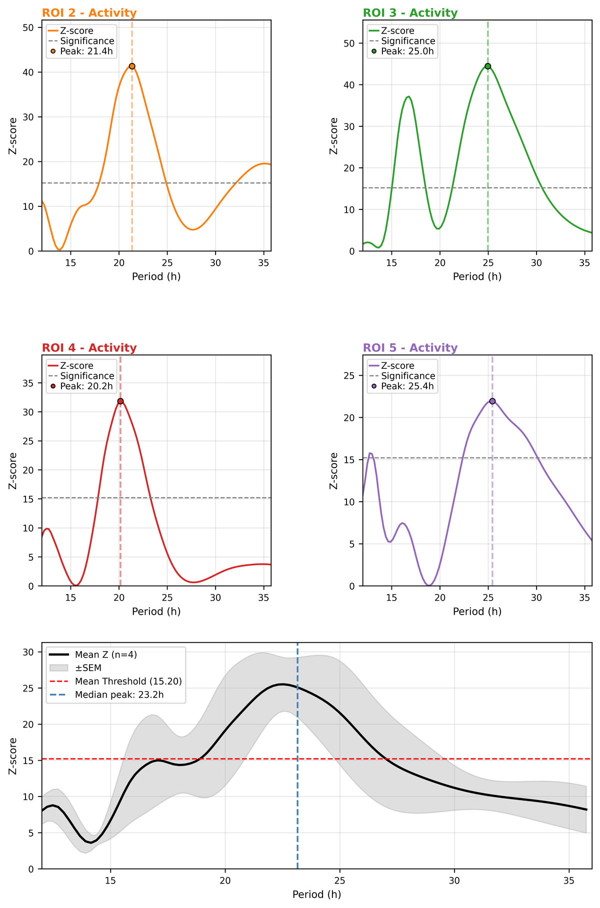
Example Chi² periodogram output: per-ROI Z(T) with the Bonferroni threshold (≈ 15.2) and the population mean (real Nematostella recording, 4 ROIs).

Chi² Statistic Plot

Note: The y-axis is labeled "Z-score" in the plot, but the quantity displayed is the chi-squared statistic Z(T) = n × (r_cos² + r_sin²), which follows χ²(df=2) under H₀.

• Blue curve: Chi-squared statistic Z(T) across all tested periods
• Gray dashed line: Bonferroni-corrected significance threshold (≈ 15.2 for α=0.05, m=100)
• Colored vertical line: Dominant period (if significant)
• Colored marker: Peak Z(T) value

Statistical Metrics

• Dominant Period: Period with highest Z(T) (hours)
• Z(T) value: Strength of rhythm (higher = stronger); labeled "Z-score" in output
• p-value: Per-test p = e^(-Z/2); significance decision uses Bonferroni threshold
• Critical Z: Bonferroni-corrected threshold ≈ 15.2 (for α=0.05, m=100 periods)

What Values Mean

Z(T) value	Bonferroni significant	Interpretation
> 20	Yes	Very strong, highly significant rhythm
15-20	Yes (near threshold)	Significant rhythm
6-15	No (below threshold)	Weak or marginal rhythm; not significant after correction
< 6	No	No significant rhythm

Example Results

ROI 1:
  ✓ Significant circadian rhythm detected (Z=125.45 > threshold 15.2)
  Dominant period: 24.12 hours
  Z(T): 125.45  (p = e^(-125.45/2) ≈ 0)

Interpretation: This ROI shows a very strong 24-hour rhythm. The chi-squared statistic (125.45) far exceeds the Bonferroni-corrected threshold (≈ 15.2), confirming significance with extremely high confidence.

Advantages

✅ Statistical Rigor - Provides p-values for objective significance testing - Chi-square distribution (df=2) is well-established - Clear yes/no answer: rhythm is significant or not

✅ Hypothesis Testing - Specifically tests for periodicity at each frequency - Ideal for confirming expected rhythms (e.g., "is there a 24h rhythm?") - Robust against noise with sufficient data

✅ Interpretability - Z-scores are intuitive (higher = stronger rhythm) - Direct biological interpretation - Easy to report in publications

✅ Sensitivity - Can detect weak rhythms with sufficient data - Works well even with moderate noise levels - Effective for irregular waveforms (non-sinusoidal)

Limitations

⚠️ Computational Cost - Slower than FFT for large datasets - Tests each period individually (100 periods = 100 tests) - Multiple comparison problem is handled by Bonferroni correction (threshold ≈ 15.2 instead of 5.99)

⚠️ Data Requirements - Requires ≥3 complete cycles for statistical power - Short recordings may not reach significance - Minimum ~10 samples needed per test

⚠️ Resolution - Period resolution depends on tested range and number of test periods - Cannot provide finer resolution than ~1% of period - May miss periods outside predefined range

⚠️ Assumptions - Assumes stationary rhythm (consistent throughout recording) - Cannot detect transient or changing rhythms - Sensitive to long-term trends (requires detrending)

⚠️ Multiple Rhythms - Reports only dominant period - May miss secondary rhythms - Harmonics can complicate interpretation

When to Use

Best For: - Confirming hypothesized rhythms (e.g., circadian studies) - Publication-quality statistical validation - Comparing rhythm strength across conditions - Detecting rhythms in noisy data

Not Ideal For: - Exploratory analysis (use FFT instead) - Very short datasets (< 3 cycles) - Rapidly changing rhythms - Identifying all frequency components simultaneously

Best Practices

1. Data Duration: Need at least 3 complete cycles for reliable detection
2. For 24h rhythms: minimum 72 hours of data

3. For 12h rhythms: minimum 36 hours of data

4. Period Range: Set based on expected rhythms

5. Circadian: 20-28 hours
6. Ultradian: 2-12 hours

7. Custom ranges for specific research questions

8. Binning: Use for high-resolution data

9. Raw data at 5-second intervals → bin to 60 seconds

10. Reduces noise while preserving rhythmic patterns

11. Multiple Comparisons: Bonferroni correction for m=100 periods is applied automatically

12. The significance threshold is χ²(1 − 0.05/100, df=2) ≈ 15.2
13. No manual correction is needed; is_significant already reflects this

---

FFT Power Spectrum

At a glance

Output: power spectrum (|FFT|², a.u.) across all frequencies + a permutation p-value.

Use for: exploring unknown or multiple rhythms and harmonics across all frequencies at once.

What It Does

Fast Fourier Transform (FFT) converts time-series data into the frequency domain, revealing all periodic components simultaneously. Unlike the Chi² periodogram which tests specific candidate periods, FFT provides a complete spectral decomposition that can reveal unexpected periodicities, harmonics, and the overall noise floor.

How It Works

1. Linear Detrending: Removes baseline drift
2. Windowing: Applies Hann window to reduce spectral leakage
3. Zero-Padding: Pads signal 4× for better frequency resolution
4. FFT Computation: Calculates power spectrum
5. Permutation Test: Assesses statistical significance
6. Peak Detection: Identifies significant frequency peaks

Mathematical details, with the code for each step

All fragments are from fft_periodogram() in _circadian_fft.py; the permutation test lives in _permutation_test_fft() in the same file.

Symbols

Symbol	Meaning	Unit
x[n]	binned activity signal, sample n = 0 … N−1	signal units
N	number of samples	—
Δt	sampling interval	s
w[n]	window function	—
NFFT	transform length after zero-padding	—
X[k]	complex DFT coefficient of bin k	signal units
P[k]	power, |X[k]|²	signal units²
fk	frequency of bin k, k/(NFFT·Δt)	Hz
Tk	period of bin k, 1/fk	s → h
φ	phase of the dominant coefficient	rad
Nperm	number of surrogates (1000)	—

---

Step 1 — linear detrending

A linear trend produces a large DC component and leaks into the low frequencies, where it can bury the circadian peak.

x_detrended[n] = x[n] − (â·n + b̂)

with â, b̂ the least-squares estimates of the trend.

detrended = signal.detrend(time_series)      # subtracts the LS straight line  (line 140)

---

Step 2 — Hann window

The DFT assumes the signal repeats with period N. A non-integer number of cycles therefore creates a discontinuity at the wrap-around, and its energy smears across neighbouring bins (spectral leakage). Tapering both ends to zero suppresses that:

w[n] = 0.5 · (1 − cos(2πn/(N−1))),   n = 0 … N−1
x_windowed[n] = x_detrended[n] · w[n]

if window == "hann":
    win = np.hanning(len(detrended))         # w[n], the raised cosine        (line 145)
detrended = detrended * win                  # element-wise taper             (line 152)

The Hann window buys ~32 dB sidelobe suppression at the cost of a slightly wider main lobe — the usual trade-off between leakage and resolution.

---

Step 3 — zero-padding

Native resolution is Δf = 1/(N·Δt). Appending zeros interpolates intermediate bins, which makes the peak easier to locate without adding information:

N_FFT = max( 2^⌈log₂(4N)⌉ , 4N )

# 4x the length, rounded up to a power of two — FFT is fastest there.
n_fft = max(2 ** int(np.ceil(np.log2(len(detrended) * 4))), len(detrended) * 4)  # (line 156)

---

Step 4 — the transform and the power spectrum

X[k] = Σₙ₌₀^(N−1) x[n] · e^(−i2πkn/N_FFT)
P[k] = |X[k]|² = Re(X[k])² + Im(X[k])²

# rfft, not fft: for a real signal the spectrum is symmetric, so only the
# bins up to Nyquist (1/2Δt) carry unique information.
fft_values = np.fft.rfft(detrended, n=n_fft)     # X[k] (complex)            (line 157)
power_spectrum = np.abs(fft_values) ** 2         # P[k]                      (line 158)

---

Step 5 — from frequency bins to periods

f_k = k / (N_FFT · Δt)          T_k = 1/f_k  (s)  → /3600  (h)

frequencies = np.fft.rfftfreq(n_fft, d=sampling_interval)   # f_k in Hz      (line 161)

# Bin 0 is the DC component: f = 0 would divide by zero, so it is masked
# out and left at period 0 instead of ∞.
periods = np.zeros_like(frequencies)                                       # (line 164)
nonzero_mask = frequencies > 0
periods[nonzero_mask] = (1.0 / frequencies[nonzero_mask]) / 3600.0         # (line 167)

# Keep only what the user asked for (e.g. the circadian 20–28 h window).
period_mask = (periods >= min_period_hours) & (periods <= max_period_hours)  # (line 170)
relevant_periods = periods[period_mask]
relevant_power = power_spectrum[period_mask]

---

Step 6 — dominant period

k_dom = argmax_k P[k]   over the selected period range

max_power_idx = np.argmax(relevant_power)          # k_dom                  (line 186)
dominant_period = relevant_periods[max_power_idx]  # T_dom                  (line 187)
dominant_frequency = relevant_freqs[max_power_idx] # f_dom                  (line 188)
dominant_power = relevant_power[max_power_idx]     # P_obs                  (line 189)

---

Step 7 — phase and peak time of the dominant component

For a cosine A·cos(2πft + φ) the rfft coefficient at f is approximately (N/2)·A·e^(iφ), so the complex angle is the phase:

φ      = arg X[k_dom]
t_peak = (−φ / (2πf_dom)) mod T_dom

relevant_indices = np.where(period_mask)[0]
dominant_fft_idx = relevant_indices[max_power_idx]   # index in the full spectrum
dominant_phase_rad = float(np.angle(fft_values[dominant_fft_idx]))   # φ     (line 199)

# Same maximum condition as in the Cosinor: the cosine peaks where its
# argument is zero, so t_peak = −φ/(2πf), folded into one cycle.
peak_time_seconds = -dominant_phase_rad / (2.0 * np.pi * dominant_frequency)  # (line 202)
dominant_peak_time_hours = float(peak_time_seconds / 3600.0) % float(dominant_period)

Hann windowing preserves phase for frequencies that fall exactly on a bin; off-bin frequencies pick up a small error, which the 4× zero-padding keeps small.

---

Step 8 — significance by permutation

FFT power has no simple analytic null distribution, so the null is built by shuffling. Shuffling destroys the temporal order while keeping the amplitude distribution, and the statistic is the maximum power over the whole tested range — which is what accounts for scanning many frequencies at once:

b = Σᵢ 𝟙[ P_perm,i ≥ P_obs ]
p = (b + 1) / (N_perm + 1)

for _ in range(n_permutations):                    # N_perm = 1000          (line 50)
    # Break the temporal structure, keep the value distribution.
    permuted = np.random.permutation(time_series)                          # (line 52)

    # Exactly the same preprocessing as the observed signal — otherwise the
    # null distribution would not be comparable.
    detrended = signal.detrend(permuted)                                   # (line 55)
    ...
    power_spectrum = np.abs(np.fft.rfft(detrended, n=n_fft)) ** 2
    period_mask = (periods >= min_period_hours) & (periods <= max_period_hours)
    permuted_powers.append(power_spectrum[period_mask].max())   # max, not one bin (line 83)

# Phipson & Smyth (2010) add-one correction: the observed statistic counts
# as one draw from the discrete null, which also prevents p = 0.
b = int(np.sum(np.array(permuted_powers) >= observed_power))               # (line 93)
p_value = (b + 1.0) / (n_permutations + 1.0)                               # (line 94)

With 1000 surrogates the smallest reachable p-value is 1/1001 ≈ 0.001 — a floor, not a measure of how strong the rhythm is.

Parameters

• Minimum Period / Maximum Period: Analysis range in hours. This is the same period-range control as the Chi² periodogram (shared spin-boxes + preset buttons), so it likewise defaults to 0.5 – 8.0 hours — use the Circadian / Auto-Detect presets for a ~24 h search.
• Window Function: Type of windowing (default: "hann")
• "hann": Good general-purpose window
• "hamming": Similar to Hann, slightly different sidelobe properties
• "blackman": Better frequency resolution, lower spectral leakage
• Bin Size: Optional data averaging

Output Interpretation

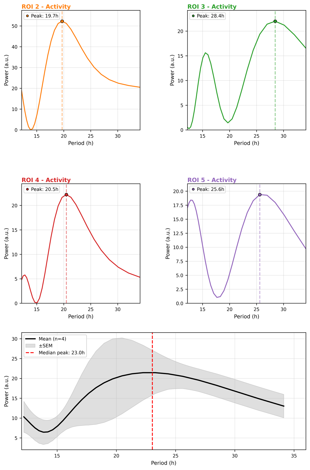
Example FFT power-spectrum output across the tested period range (real Nematostella recording).

Power Spectrum Plot

• Colored curve: Power across all frequencies
• Colored vertical line: Dominant period
• Colored marker: Peak power value

Spectral Metrics

• Dominant Period: Period with maximum power (hours)
• Dominant Power: Strength at dominant frequency
• Frequency Peaks: List of all significant peaks (period, power)

Power Values

Power is in arbitrary units (AU²). Relative values matter more than absolute values:

Relative Power	Interpretation
10× higher than others	Very strong dominant rhythm
2-5× higher	Clear rhythm
Similar to others	Weak or multiple competing rhythms

Comparison with Chi² Periodogram

Feature	Chi² Periodogram	FFT
Output	Bonferroni-corrected Z(T) statistic	Power spectrum (
Strength	Tests specific hypotheses, built-in correction	Explores all frequencies simultaneously
Significance	Bonferroni-corrected threshold ≈ 15.2	Permutation p-value (max-power test)
Use Case	Confirm expected rhythms with rigorous correction	Discover unknown rhythms

Agreement: Both should identify the same dominant period. Typical differences: - Chi² Periodogram: 24.0h - FFT: 23.7-24.3h (slightly different due to frequency resolution)

Differences < 1 hour indicate excellent agreement.

Advantages

✅ Computational Efficiency - Very fast (O(N log N) algorithm) - Analyzes all frequencies simultaneously - Scales well to large datasets

✅ Exploratory Power - Reveals all periodic components at once - No need to specify expected periods in advance - Identifies harmonics and secondary rhythms automatically

✅ Standard Method - Widely used in signal processing - Extensive literature and validation - Compatible with other spectral analysis tools

✅ Visual Clarity - Power spectrum shows full frequency content - Easy to identify dominant peaks - Reveals complex rhythmic structures

✅ Resolution - Zero-padding provides excellent frequency resolution - Can distinguish closely-spaced periods - Continuous spectrum (not limited to discrete test periods)

Limitations

⚠️ Arbitrary Units - Power values are |FFT|² — arbitrary units (a.u.) that depend on signal amplitude and n - Absolute power values are not comparable across recordings with different durations or amplitudes - Use relative values (peak vs. background) and permutation p-values for interpretation

⚠️ Spectral Leakage - Non-integer number of cycles causes frequency spreading - Windowing reduces but doesn't eliminate leakage - Can create artificial side lobes in spectrum

⚠️ Harmonics Confusion - Strong fundamental generates harmonics (2×, 3× frequency) - Harmonics can be mistaken for independent rhythms - Example: 24h rhythm creates peaks at 12h, 8h, 6h

⚠️ Amplitude Sensitivity - Assumes sinusoidal oscillations - Non-sinusoidal waveforms spread power across frequencies - Square waves or sharp transitions create many harmonics

⚠️ Detrending Required - Very sensitive to linear trends - DC component (zero frequency) can dominate spectrum - Long-term drift must be removed

⚠️ Edge Effects - Beginning and end of recording affect spectrum - Windowing reduces but impacts amplitude estimates - Very short recordings have poor frequency resolution

When to Use

Best For: - Exploratory analysis (unknown rhythms) - Identifying multiple periodic components - Comparing spectral signatures across conditions - Fast screening of many ROIs - Detecting harmonics and complex rhythms

Not Ideal For: - When an analytic p-value is required (permutation test gives p-values but with minimum p = 0.001) - When absolute power values are needed (units are arbitrary) - Very short recordings with insufficient frequency resolution

Best Practices

1. Window Selection:
2. Hann: Default, good for most cases
3. Blackman: Use for noisy data (better spectral leakage suppression)
4. Hamming: Similar to Hann, slightly different sidelobe properties

5. None: Only for very clean periodic signals with integer cycles

6. Zero-Padding: Automatically applied (4× padding)

7. Improves frequency resolution without adding information
8. Provides smooth interpolation between frequency bins

9. Does not increase statistical power

10. Interpretation:

11. Look for clear peaks above background noise floor
12. Multiple peaks may indicate harmonics (e.g., 24h and 12h, 8h, 6h)
13. Broad peaks suggest irregular or variable-period rhythms

14. Check if secondary peaks are harmonics (integer divisors of dominant)

15. Validation:

16. Always cross-validate with the Chi² periodogram
17. Both methods should agree on dominant period (±1 hour)
18. Use Chi² periodogram for Bonferroni-corrected statistical confirmation

---

Cosinor Analysis

At a glance

Output: MESOR, Amplitude and Acrophase with 95% CIs and an F-test (plus a population Nelson F-test).

Use for: quantifying a known-period rhythm and comparing rhythm parameters between groups.

What It Does

Cosinor analysis quantifies circadian rhythms by fitting a cosine curve to activity data and extracting key rhythmic parameters: MESOR (mean level), Amplitude (rhythm strength), and Acrophase (peak timing). This is the gold standard method in chronobiology for rhythm characterization.

Mathematical details, with the code for each step

The Cosinor Model

The single-cosinor model assumes activity follows a sinusoidal pattern:

x(t) = M + A × cos(2πt/T + φ) + ε

Where: - M (MESOR): Midline Estimating Statistic Of Rhythm—the rhythm-adjusted mean level - A (Amplitude): Half the peak-to-trough difference—rhythm strength - φ (Acrophase): Phase angle at peak activity—timing within cycle - T (Period): Duration of one complete cycle (e.g., 24h for circadian) - ε: Residual error (assumed i.i.d. normal)

Linearization for Least-Squares Estimation

Direct estimation of A and φ would require nonlinear optimization. Using the trigonometric identity cos(θ+φ) = cos(θ)cos(φ) - sin(θ)sin(φ), the model becomes linear:

x(t) = β₀ + β₁×cos(ωt) + β₂×sin(ωt) + ε

where ω = 2π/T, and: - β₀ = M (MESOR) - β₁ = A×cos(φ) - β₂ = -A×sin(φ)

# cosinor_analysis(), _cosinor_analysis.py
# T is fixed (from the periodogram or the period field), not fitted.
omega = 2 * np.pi / period_hours          # ω = 2π/T, rad per hour     (line 107)

Ordinary Least Squares (OLS) Estimation

Construct the n×3 design matrix:

X = | 1   cos(ωt₁)   sin(ωt₁) |
    | 1   cos(ωt₂)   sin(ωt₂) |
    | ⋮      ⋮          ⋮     |
    | 1   cos(ωtₙ)   sin(ωtₙ) |

The OLS estimator is:

β̂ = (X'X)⁻¹X'x

where x = [x(t₁), ..., x(tₙ)]' is the observation vector.

# One row per timepoint, three columns — one per unknown. The all-ones
# column is why β₀ comes out as the intercept, i.e. the MESOR.
X = np.column_stack(                                                  # (line 114)
    [
        np.ones(len(time_clean)),      # → β₀ (MESOR)                 (line 116)
        np.cos(omega * time_clean),    # → β₁                         (line 117)
        np.sin(omega * time_clean),    # → β₂                         (line 118)
    ]
)

# lstsq solves the normal equations for us — because the model is linear
# in β this is the exact optimum, with no iteration and no starting guess.
beta, residuals, rank, s = np.linalg.lstsq(X, data_clean, rcond=None) # (line 124)

Parameter Recovery:

M = β̂₀
A = √(β̂₁² + β̂₂²)
φ = atan2(-β̂₂, β̂₁)

The four-quadrant arctangent (atan2) correctly resolves phase to (-π, π] regardless of coefficient signs. Convert to clock time: t_acro = (φ/ω) mod T.

mesor = beta[0]      # β₀ = M                                         (line 127)
beta_cos = beta[1]   # β₁                                             (line 128)
beta_sin = beta[2]   # β₂                                             (line 129)

# β₁ = A·cosφ and β₂ = −A·sinφ: the two coefficients are the Cartesian
# form of one vector — length = amplitude, angle = phase.
amplitude = np.sqrt(beta_cos**2 + beta_sin**2)                        # (line 135)
# The minus sign on β₂ undoes the sign in β₂ = −A·sinφ.
phase_angle_rad = np.arctan2(-beta_sin, beta_cos)                     # (line 136)

# cos(ωt + φ) peaks where its argument is zero → t = −φ/ω. The modulo
# folds it into the first cycle, so this is the *first* fitted peak.
peak_time = (-phase_angle_rad / omega) % period_hours                 # (line 140)

Significance Testing (F-test)

The null hypothesis H₀: A = 0 (no rhythm) is tested by comparing the full model to the mean-only model:

F = [(SS_tot - SS_res)/k] / [SS_res/(n-k-1)] = [SS_model/2] / [SS_res/(n-3)]

where: - SS_tot = Σᵢ(xᵢ - x̄)² — total sum of squares - SS_res = Σᵢ(xᵢ - x̂ᵢ)² — residual sum of squares - SS_model = SS_tot - SS_res — model sum of squares - k = 2 — number of model parameters (cos and sin coefficients) - n-3 — residual degrees of freedom

Under H₀, F follows an F-distribution with (2, n-3) degrees of freedom.

n = len(data_clean)
k = 2                                    # cos + sin                  (line 166)
df_model = k                             # dfn = 2                    (line 167)
df_residual = n - k - 1                  # dfd = n − 3 (β₀ costs one)  (line 168)

mse_residual = ss_res / df_residual      # SS_res/(n−3)               (line 171)
mse_model = (ss_tot - ss_res) / df_model # SS_model/2                 (line 172)
f_statistic = mse_model / mse_residual   # F                          (line 173)
p_value = 1 - stats.f.cdf(f_statistic, df_model, df_residual)         # (line 174)

With thousands of frames df_residual is huge and p becomes tiny even for weak rhythms — which is why R² and Amplitude carry the biological statement, not p.

Goodness of Fit:

R² = 1 - SS_res/SS_tot = SS_model/SS_tot

R² represents the proportion of variance explained by the fitted sinusoid.

# SS_res: what the fitted cosine failed to explain ...
ss_res = np.sum((data_clean - (mesor                                  # (line 150)
                               + beta_cos * np.cos(omega * time_clean)
                               + beta_sin * np.sin(omega * time_clean))) ** 2)
# ... SS_tot: what a flat line at the mean would leave unexplained.
ss_tot = np.sum((data_clean - np.mean(data_clean)) ** 2)              # (line 161)
r_squared = 1 - (ss_res / ss_tot)                                     # (line 162)

The denominator is the same for every tested period, which is what makes R² comparable across the multi-period scan.

Confidence Intervals

Standard errors are computed from the variance-covariance matrix:

Var(β̂) = σ̂² × (X'X)⁻¹,    where σ̂² = SS_res/(n-3)

For MESOR: SE(M) = √Var(β̂₀)

mse = ss_res / df_residual                     # σ̂²                    (line 183)
XtX_inv = np.linalg.inv(X.T @ X)               # (X'X)⁻¹               (line 185)
var_beta = mse * np.diag(XtX_inv)              # Var(β̂), diagonal only (line 186)
se_beta = np.sqrt(var_beta)                    # SE(β̂)                 (line 187)

t_crit = stats.t.ppf(1 - alpha / 2, df_residual)                      # (line 190)
ci_mesor = (mesor - t_crit * se_beta[0], mesor + t_crit * se_beta[0]) # (line 191)

For Amplitude (nonlinear function), use the delta method:

SE(A) ≈ (1/A) × √[β̂₁²×Var(β̂₁) + β̂₂²×Var(β̂₂)]

Confidence intervals: θ ± t_{n-3,1-α/2} × SE(θ)

Population-Mean Cosinor (Nelson et al. 1979)

For multiple individuals (ROIs), the population cosinor uses the Nelson et al. (1979) F-test. Each individual ROI's OLS fit produces β_cos,j and β_sin,j. The population-level hypothesis H₀: mean(β_cos) = mean(β_sin) = 0 is tested with:

F(dfn=2, dfd=2(n−1))

where n = number of ROIs. The numerator is built from the mean β_cos and mean β_sin across all ROIs; the denominator uses the variance of those coefficients. This tests whether the population as a whole oscillates — not merely whether individual ROIs oscillate.

Population amplitude and acrophase are derived via vector averaging of individual (Aⱼ, φⱼ):

xⱼ = Aⱼ×cos(φⱼ),    yⱼ = Aⱼ×sin(φⱼ)
x̄ = (1/J)Σⱼxⱼ,    ȳ = (1/J)Σⱼyⱼ
A_pop = √(x̄² + ȳ²),    φ_pop = atan2(ȳ, x̄)

Output Parameters

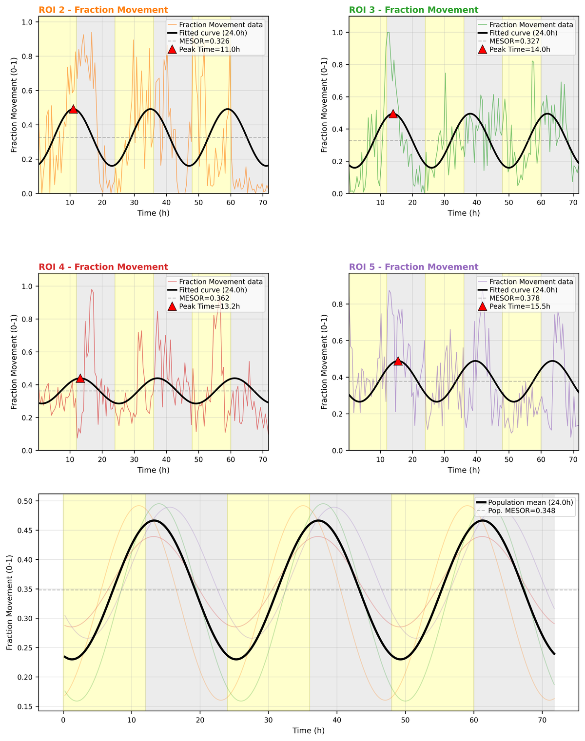
Example cosinor output: fitted cosine curves overlaid on the activity data (real Nematostella recording).

Individual ROI Results: - Best-fit period: Period with highest R² among tested periods - MESOR: Mean activity level (rhythm-adjusted baseline) - Amplitude: Strength of rhythm (0 = no rhythm, higher = stronger) - Acrophase: Time of peak activity (hours from recording start) - R²: Goodness of fit (>0.3 = strong rhythm, 0.1-0.3 = moderate, <0.1 = weak) - p-value: Statistical significance (p < 0.05 = significant rhythm) - 95% Confidence Intervals: Uncertainty ranges for each parameter

Population Results: - Population MESOR: Average baseline activity across all ROIs - Population Amplitude: Collective rhythm strength (vector-averaged) - Population Acrophase: Common peak time across population - Proportion significant: Percentage of ROIs with significant rhythms

Interpretation Guide

MESOR (Midline Estimating Statistic of Rhythm)

• What it means: The rhythm-adjusted mean activity level
• Typical values: 0.0-1.0 (fraction movement data)
• Interpretation:
• High MESOR (>0.5): Generally active organism
• Low MESOR (<0.2): Generally inactive organism
• MESOR ≠ simple mean (accounts for rhythmic variation)

Amplitude

• What it means: Half the distance between peak and trough
• Typical values: 0.0-0.5 for fraction movement
• Interpretation:
• High amplitude (>0.2): Strong, robust circadian rhythm
• Moderate amplitude (0.1-0.2): Detectable but weaker rhythm
• Low amplitude (<0.1): Weak or absent rhythm
• Amplitude = 0: Arrhythmic (constant activity level)

Clinical relevance: - Aging typically reduces amplitude (rhythm fragmentation) - SCN lesions eliminate amplitude (no circadian clock) - Zeitgebers (light/dark) increase amplitude (entrainment)

Acrophase

• What it means: Time of peak activity within the cycle
• Units: Hours from start of recording
• Interpretation:
• For 24h rhythm with lights on at t=0:
  • Acrophase = 8-12h: Diurnal (day-active)
  • Acrophase = 20-24h or 0-4h: Nocturnal (night-active)
• Acrophase shift indicates:
  • Phase advance: Peak occurs earlier (e.g., jet lag west→east)
  • Phase delay: Peak occurs later (e.g., jet lag east→west)

Group comparisons: - Synchronized population: Similar acrophases (low SD) - Desynchronized population: Variable acrophases (high SD) - Anti-phase relationship: Acrophases differ by ~12h (for 24h rhythm)

R² (Goodness of Fit)

• What it means: Proportion of variance explained by the cosine model
• Scale: 0.0-1.0
• Interpretation:
• R² > 0.5: Excellent fit, very strong rhythm
• R² = 0.3-0.5: Good fit, strong rhythm
• R² = 0.1-0.3: Moderate fit, detectable rhythm
• R² < 0.1: Poor fit, weak or no rhythm

Why R² matters: - High R²: Activity closely follows cosine pattern (clean rhythm) - Low R²: Activity deviates from cosine (ultradian, noise, or arrhythmic) - Compare with p-value: significant but low R² = detectable but weak rhythm

p-value

• What it tests: Null hypothesis that amplitude = 0 (no rhythm)
• Interpretation:
• p < 0.001 (***): Very strong evidence for rhythm
• p < 0.01 (**): Strong evidence for rhythm
• p < 0.05 (*): Significant rhythm detected
• p ≥ 0.05 (ns): No significant rhythm

Important notes: - Large sample sizes can yield p < 0.05 with low amplitude (biological significance ≠ statistical) - Check R² and amplitude together with p-value - Confidence intervals show precision of estimates

When to Use Cosinor

Ideal scenarios: - Quantifying rhythm strength: Need numeric amplitude and MESOR values - Comparing experimental groups: Test if treatment affects rhythm parameters - Publication requirements: Cosinor is the most widely accepted method in chronobiology - Known period: Testing specific periods (e.g., 24h circadian rhythm) - Population studies: Combining rhythms across multiple individuals - Phase response curves: Measuring acrophase shifts after zeitgeber pulses

Advantages: - Provides interpretable, quantitative parameters (MESOR, Amplitude, Acrophase) - Statistical testing with p-values and confidence intervals - Fast computation (least squares regression) - Robust to moderate noise - Standard method in chronobiology literature (easy comparison with published work) - Population-level statistics available

Limitations: - Assumes sinusoidal rhythm (cosine wave) - may miss complex waveforms - Single-component model (doesn't detect multiple simultaneous rhythms like FFT) - Requires ~2-3 complete cycles for reliable parameter estimation - Less suitable for exploratory analysis (need to specify test periods) - Cannot detect period if not in the tested range

Practical Example

Scenario: Testing whether a mutation affects circadian rhythm strength

Wildtype (WT) results:

ROI 1:
  Best-fit period: 24.0 hours
  MESOR: 0.35 (moderate baseline activity)
  Amplitude: 0.25 (strong rhythm)
  Acrophase: 14.2 hours (peak in mid-afternoon)
  R²: 0.65 (good fit)
  p-value: 0.0001 (***)

Population:
  Amplitude: 0.23 (consistent across animals)
  All 6 ROIs significant (100%)

Mutant results:

ROI 1:
  Best-fit period: 24.0 hours
  MESOR: 0.34 (similar baseline to WT)
  Amplitude: 0.08 (weak rhythm - 3× lower than WT!)
  Acrophase: 16.5 hours (2h phase delay)
  R²: 0.18 (poor fit)
  p-value: 0.12 (ns)

Population:
  Amplitude: 0.06 (very weak)
  Only 2/6 ROIs significant (33%)

Interpretation: Mutation causes circadian rhythm disruption: - Amplitude reduced by 68% (from 0.25 to 0.08) - Most individuals show no significant rhythm (100% → 33%) - MESOR unchanged (mutation affects clock, not overall activity) - Acrophase variable (desynchronization)

Conclusion: Mutation impairs circadian clock function without affecting total activity levels. This would be missed by standard activity analysis but clearly detected by cosinor.

Comparison with Other Methods

Feature	Cosinor	Chi² Periodogram	FFT
Primary Use	Quantify rhythm parameters	Detect significant periods	Explore all frequencies
Output	MESOR, Amplitude, Acrophase	Z(T) with Bonferroni threshold; Nelson F for population	Power spectrum (
Best for	Known periods, group comparisons	Period detection, Bonferroni-corrected testing	Exploratory analysis
Speed	Very fast	Slow	Very fast
Statistics	p-values + 95% CIs; Nelson F-test	Bonferroni-corrected Z(T) threshold	Permutation p-values (max-power test)
Assumptions	Sinusoidal rhythm	None (non-parametric)	Stationarity

Recommendation: Use Cosinor for quantifying known rhythms (e.g., testing 24h circadian), Chi² Periodogram for detecting unknown periods with Bonferroni-corrected statistical validation, and FFT for broad exploratory analysis of all frequencies.

Tips and Best Practices

1. Period Selection:
2. Test biologically relevant periods: 12h (ultradian), 24h (circadian), 30h (infradian)
3. Include period range based on recording duration

4. For free-running conditions, test 20-28h (circadian period may not be exactly 24h)

5. Data Requirements:

6. Minimum: 2 complete cycles (48h for circadian)
7. Recommended: ≥3 cycles (72h for circadian)

8. Longer recordings improve parameter precision (tighter confidence intervals)

9. Interpreting Significance:

10. p < 0.05 but R² < 0.1: Statistically detectable but biologically weak rhythm
11. p ≥ 0.05 but R² > 0.2: May be underpowered, try longer recording

12. High amplitude with high p-value: Check for outliers or bimodal rhythm

13. Population Analysis:

14. If <50% of individuals significant: population-level rhythm questionable
15. High variability in acrophases: desynchronized population

16. Use vector plots to visualize population phase distribution

17. Validation:

18. Always plot fitted curves over raw data (visual inspection critical)
19. Check that acrophase aligns with visible peaks

20. Compare results with Chi² periodogram or FFT for consistency

21. Common Pitfalls:

22. Testing too many periods: Multiple comparison problem (adjust α or use best-fit)
23. Ignoring confidence intervals: Wide CIs indicate imprecise estimates
24. Over-interpreting small amplitude: Amplitude < 0.05 may be noise, even if significant

---

ROI Similarity Matrix

At a glance

Output: a pairwise signed correlation matrix (lag window ±3 h), the optimal lag per pair, and UPGMA clusters.

Use for: finding synchronized or anti-phase ROI groups (social structure, dominance).

What It Does

Computes pairwise cross-correlations between all ROIs to identify synchronized or anti-phase activity patterns. Uses hierarchical clustering to group similar ROIs. Provides both a similarity metric and phase offset estimates.

How It Works

1. Normalization: Standardizes each ROI's activity (mean=0, std=1)
2. Cross-Correlation: Calculates correlation at different time lags (±12 h)
3. Similarity value: takes the signed correlation from a narrow window around lag 0 (±3 h by default) — the value the matrix and the clustering use
4. Peak Detection: additionally reports the maximum over the full ±12 h scan and its lag (descriptive)
5. Significance Testing: t-test on the similarity value
6. Clustering: Groups ROIs by similarity using hierarchical clustering, distance d = (1 − r)/2

Changed on 2026-09-23 — what and why

Before: the matrix stored max_correlation, the maximum of the signed correlation over the whole ±12 h lag scan, and the clustering used d = 1 − r.

The problem: for a circadian signal, lag and phase are circular. A window of ±12 h is half a period at T = 24 h, so every phase relationship is reachable inside it — an anti-phase pair peaks at ±12 h and is numerically indistinguishable from a synchronous pair with a lag. Two consequences followed:

• Anti-phase animals entered the matrix with a positive r and were merged into the same cluster as the synchronous ones. The one pairwise statement this method could make — who runs with whom and who against — was lost. (Whether both are rhythmic at the same period is what the Coherence Analysis already answers.)
• The reported optimal lag pinned to the window edge: at T = 26 h the anti-phase maximum lies at 13 h, outside the window, so the scan returned a truncated edge value that reads like a measurement.

Now: the matrix value is the signed correlation from a narrow window (±3 h, parameter similarity_lag_hours) — wide enough for the phase spread within one chronotype, far too narrow for anti-phase to fold in. The clustering maps r → d = (1 − r)/2, so +1 → 0, 0 → 0.5, −1 → 1: an anti-phase pair now sits at the far end of the dendrogram. The full ±12 h scan is still computed and returned as full_scan_correlation_matrix / full_scan_lag_matrix.

Why not simply take the largest |r| over the full scan? For an anti-phase pair |r| is equally large at lag 0 and at ±12 h. argmax would hit a tie and pick whichever index comes first — the lag would become arbitrary, not more correct.

Measured on synthetic traces (24 h cosine, 3 days, 10 min bins):

Pair	matrix value now	old full-scan value
2 h apart, same phase	+0.98 at −1.8 h	+0.98 at −1.8 h
anti-phase	−1.00 at 0 h	+1.00 at −11.8 h
rhythmic vs. noise	−0.08	+0.09 at +11.5 h (edge)

Clustering at r ≥ 0.5 groups the first pair and separates the anti-phase animal; with the old values all three ended up in one cluster.

The rebuild also removed an impossible value: the per-lag normalisation by n − |τ| can overshoot slightly at large lags, and the old matrix contained entries up to r = 1.03. Distances derived from those were negative and made scipy.cluster.hierarchy reject the linkage. The similarity value is now clipped to [−1, 1].

Mathematical details, with the code for each step

All fragments are from _circadian_similarity.py: steps 1–4 from calculate_cross_correlation(), step 5 from correlation_significance_test(), step 7 from hierarchical_clustering().

Symbols

Symbol	Meaning	Unit
x(t), y(t)	activity traces of two ROIs	signal units
x̃, ỹ	z-standardised traces (mean 0, sd 1)	—
n	number of samples per trace	—
τ	lag between the two traces	samples → h
rxy(τ)	cross-correlation at lag τ	—
rmax, τopt	peak correlation and the lag where it occurs	—, h
t	t-statistic of the correlation	—
ν	degrees of freedom, n−2	—
N	number of ROIs	—
dij	distance between ROI i and j, 1 − rij	—

---

Step 1 — standardise both traces

x̃(t) = (x(t) − x̄) / σₓ          ỹ(t) = (y(t) − ȳ) / σᵧ

# +1e-10 guards against a flat trace (σ = 0) turning the result into NaN.
s1 = (signal1 - np.mean(signal1)) / (np.std(signal1) + 1e-10)              # (line 130)
s2 = (signal2 - np.mean(signal2)) / (np.std(signal2) + 1e-10)              # (line 131)

Standardising is what makes the result a correlation rather than a covariance: absolute activity level and scale drop out, only the shape of the time course is compared.

---

Step 2 — raw cross-correlation over all lags

c(τ) = Σₜ x̃(t) · ỹ(t+τ)

n = len(s1)
# scipy returns the raw dot-product sum per lag, not yet normalised.
correlation = signal.correlate(s1, s2, mode="same", method="auto")         # (line 135)

---

Step 3 — restrict to ±12 h of lag

A circadian pair can be at most half a period apart before "late" becomes "early", so the search window is capped:

τ_max = min( 12 h / Δt , (len(c) − 1) / 2 )      in samples

max_lag_samples = int((max_lag_hours * 3600) / sampling_interval)          # (line 143)
# Clamp so the window stays inside the array on both sides.
max_lag_samples = min(max_lag_samples, (len(correlation) - 1) // 2)        # (line 144)

center = len(correlation) // 2                    # zero lag sits here     (line 146)
lag_range = slice(center - max_lag_samples, center + max_lag_samples + 1)
correlation_window = correlation[lag_range].copy()
lag_hours = lag_samples * sampling_interval / 3600.0   # τ in hours        (line 151)

---

Step 4 — unbiased normalisation per lag

At lag τ only n − |τ| sample pairs actually overlap. Dividing by the full n would shrink the large-lag values artificially, so each lag is divided by its own overlap count:

r_xy(τ) = c(τ) / (n − |τ|)

for idx, k in enumerate(lag_samples):                                     # (line 156)
    n_overlap = n - abs(int(k))          # overlapping pairs at this lag   (line 157)
    if n_overlap > 0:
        correlation_window[idx] /= n_overlap
    else:
        correlation_window[idx] = 0.0

This is what keeps r inside [−1, 1] and comparable across lags.

---

Step 5 — the similarity value (what the matrix stores)

r_sim = r_xy(τ*)   with   τ* = argmax_{|τ| ≤ 3 h} |r_xy(τ)|      (sign kept)

# Narrow window around lag 0: wide enough for the phase spread within one
# chronotype, far too narrow for anti-phase (±T/2) to fold in.
similarity_mask = np.abs(lag_hours) <= float(similarity_lag_hours)
similarity_idx_local = np.argmax(np.abs(correlation_window[similarity_mask]))
similarity_idx = np.where(similarity_mask)[0][similarity_idx_local]

# Clipped because the (n − |k|) normalisation is only approximately a
# Pearson r and can overshoot at large lags; the clustering needs a value
# in [−1, 1] to produce distances in [0, 1].
similarity_correlation = float(np.clip(correlation_window[similarity_idx], -1.0, 1.0))
similarity_lag = lag_hours[similarity_idx]

The sign is kept: an anti-phase pair stays at r ≈ −1 instead of reappearing as a positive peak half a period away.

---

Step 6 — full-scan maximum (reported, not used for clustering)

r_max = max_τ r_xy(τ)          τ_opt = argmax_τ r_xy(τ)      over ±12 h

# Descriptive only — see the "Changed on 2026-09-23" box above for why this
# value must not drive the matrix.
max_corr_idx = np.argmax(correlation_window)
max_correlation = correlation_window[max_corr_idx]     # r_max
optimal_lag = lag_hours[max_corr_idx]                  # τ_opt in hours

Pairs with |τ_opt| < 1 h count as in-phase.

---

Step 7 — significance of one pair

Under H₀: ρ = 0,

t = r · √[(n−2) / (1−r²)]        ν = n − 2
p = 2 · (1 − F_t,ν(|t|))                       (two-tailed)
r_crit = √[ t²_crit / (n − 2 + t²_crit) ]      with t_crit = F⁻¹_t,ν(1 − α/2)

The test runs on the similarity value, i.e. on the number the matrix and the dendrogram show.

t_stat = r * np.sqrt((n - 2) / (1 - r**2))          # t                    (line 72)
# Two-tailed: a strong anti-correlation is just as much a finding.
p_value = 2 * (1 - stats.t.cdf(abs(t_stat), df=n - 2))                     # (line 75)

r_crit falls as n grows — with tens of thousands of frames even a tiny correlation clears the threshold, which is why the matrix should be read by effect size, not by significance stars alone.

---

Step 8 — Bonferroni across all pairs, then clustering

With N ROIs there are N(N−1)/2 simultaneous tests:

α_corr = α / n_pairs,     n_pairs = N(N−1)/2
d_ij   = (1 − r_ij) / 2              correlation → distance

# (1 - r)/2 maps +1 → 0, 0 → 0.5, -1 → 1, so an anti-phase pair sits at the
# far end of the tree instead of being merged with the synchronous ones.
# Single-sourced in correlation_to_distance() so the dendrogram cut line
# and the clustering cannot drift apart.
distance_matrix = correlation_to_distance(correlation_matrix)
np.fill_diagonal(distance_matrix, 0)

# scipy wants the condensed (upper-triangle) form.
condensed_dist = squareform(distance_matrix, checks=False)                 # (line 381)

# Average linkage = UPGMA: merge the two clusters with the smallest mean
# inter-cluster distance.
linkage_matrix = hierarchy.linkage(condensed_dist, method=method)          # (line 384)

# Cut at d = (1 - r)/2; the GUI slider sets r, the default is r = 0.5,
# i.e. a cut at d = 0.25.
cluster_labels = hierarchy.fcluster(linkage_matrix, t=threshold, criterion="distance")

Important: the clustering is exploratory and descriptive. Cluster assignments are not tested; significance claims belong to the Bonferroni-corrected pairwise correlations.

Parameters

• Maximum Lag: Maximum time shift to test (default: 12 hours)

Output Interpretation

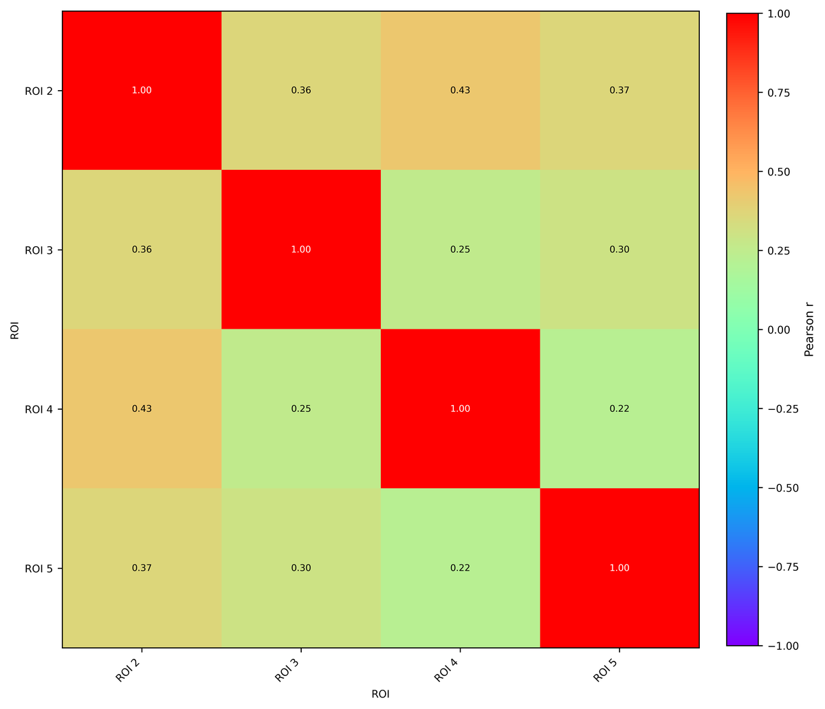
Example ROI-similarity output: the pairwise cross-correlation matrix (real Nematostella recording).

Correlation Matrix Heatmap

• Green: High positive correlation (synchronized)
• Yellow: Low correlation (independent)
• Red: Negative correlation (anti-phase)

Correlation	Lag	Interpretation
> 0.9	0	Perfect synchronization
0.7-0.9	0	Strong synchronization
0.5-0.7	0	Moderate synchronization
0.7-0.9	½ period	Anti-phase relationship
< 0.3	any	Independent/unrelated

Dendrogram (Hierarchical Clustering)

• Height: Dissimilarity d = 1 − r
• Branches: ROIs that cluster together
• Colors: Different clusters (automatically split at the threshold)
• Red dashed line: Cluster threshold from the GUI slider (default r = 0.5 → d = 0.5)

Similarity Table

For each ROI pair: - Correlation: Strength of relationship (-1 to +1) - Lag (hours): Time offset for maximum correlation - Similarity: Percentage (0-100%)

Example Results

High Similarity Pairs:
  ROI 1 ↔ ROI 2: r=0.98, lag=0.0h (98% similar, synchronized)
  ROI 3 ↔ ROI 4: r=0.95, lag=0.1h (95% similar, nearly synchronized)

Moderate Similarity:
  ROI 1 ↔ ROI 3: r=0.82, lag=12.0h (anti-phase, same period)

Low Similarity:
  ROI 1 ↔ ROI 5: r=0.35, lag=2.1h (independent rhythms)

Clustering Interpretation

Group A (ROIs 1-2): Synchronized 24h rhythm Group B (ROIs 3-4): Synchronized 24h rhythm, anti-phase to Group A Group C (ROIs 5-6): Different period (20h rhythm)

Advantages

✅ Lag Detection - Automatically finds optimal time offset for maximum correlation - Detects anti-phase relationships (phase-shifted rhythms) - Reveals sequential behaviors (e.g., dominance hierarchies)

✅ Visual Clarity - Heatmap provides immediate overview of all pairwise relationships - Dendrogram shows natural groupings - Easy to identify synchronized clusters

✅ Normalization - Correlation coefficient (-1 to +1) is standardized - Independent of absolute activity levels - Allows fair comparison between ROIs with different amplitudes

✅ Clustering - Hierarchical clustering automatically groups similar ROIs - Objective grouping based on similarity threshold - Reveals social structure and behavioral coordination

✅ Comprehensive - Analyzes all possible pairs simultaneously - Single analysis provides complete synchronization picture - Useful for exploratory analysis

Limitations

⚠️ Period Assumption - Assumes all ROIs have similar period lengths - Cannot distinguish "same period, different phase" from "different periods" - Mixed periods (e.g., 20h and 24h) show artificially low correlation

⚠️ Computational Cost - O(N²) pairs for N ROIs (6 ROIs = 15 pairs, 20 ROIs = 190 pairs) - Cross-correlation at each lag is computationally intensive - Large datasets with many ROIs can be slow

⚠️ Lag Interpretation - Lag values can be ambiguous (e.g., +6h vs -18h in 24h cycle) - Maximum lag parameter affects results - Anti-phase may appear as high positive correlation at large lag

⚠️ Stationarity Requirement - Assumes consistent relationship throughout recording - Transient synchronization events are averaged out - Cannot detect changes in coordination over time

⚠️ No Frequency Information - Overall correlation doesn't specify which frequencies are synchronized - High correlation could be due to any shared frequency component - Cannot distinguish circadian vs ultradian synchronization

⚠️ Sensitivity to Noise - Random noise reduces correlation coefficients - May fail to detect weak synchronization - Short recordings amplify noise effects

When to Use

Best For: - Identifying synchronized groups (social clusters) - Detecting phase relationships (in-phase vs anti-phase) - Comparing overall behavioral similarity - Finding dominant hierarchies (lag-based sequences) - Exploratory analysis of social structure

Not Ideal For: - Mixed-period datasets (different rhythm frequencies) - Frequency-specific synchronization (use Coherence instead) - Very short recordings (< 2 cycles) - When timing precision is critical - Transient or changing synchronization

Best Practices

1. Lag Selection:
2. Set to ½ of maximum expected period
3. For 24h rhythms: 12-hour lag captures anti-phase
4. Too small: May miss anti-phase relationships

5. Too large: Increases computation time

6. Cluster Interpretation:

7. Tight clusters (height < 0.3): Very similar behavior
8. Loose clusters (height > 0.7): Weakly related
9. Isolated branches: Unique patterns

10. Compare with domain knowledge (e.g., known social groups)

11. Biological Meaning:

12. High correlation + zero lag → Social synchronization, shared zeitgeber
13. High correlation + non-zero lag → Sequential behavior, dominance
14. Anti-phase (r < 0 or lag ≈ ½ period) → Competition, resource partitioning

15. Low correlation → Independent rhythms, different periods, or no coordination

16. Validation:

17. Cross-check with Coherence analysis
18. Verify period similarity with Chi²/FFT first
19. Consider biological context (social species vs solitary)

---

Coherence Analysis

At a glance

Output: frequency-specific magnitude-squared coherence γ²(f) for every ROI pair.

Use for: detecting a shared rhythm at a specific frequency even when signals are phase-shifted.

What It Does

Measures frequency-specific synchronization between ROI pairs using Welch's method. Unlike cross-correlation (which measures overall similarity), coherence identifies which specific frequency components are synchronized. Two ROIs might have low overall correlation but high coherence at the circadian frequency.

How It Works

1. Welch's Method: Divides data into overlapping segments for robust spectral estimation
2. Spectral Density Estimation: Computes auto- and cross-spectral densities
3. Coherence Calculation: Normalizes to 0-1 scale at each frequency
4. Significance Testing: Compares to threshold based on number of segments

Mathematical details, with the code for each step

All fragments are from calculate_coherence() in _circadian_coherence.py; the threshold lives in coherence_significance_threshold() in the same file.

Symbols

Symbol	Meaning	Unit
L	segment length (nperseg)	samples
K	number of averaged Welch segments	—
Xk[f], Yk[f]	DFT of segment k of either signal	signal units
P̂11, P̂22	auto-spectral densities	signal units²
P̂12	cross-spectral density	signal units²
γ²(f)	magnitude-squared coherence at f	— (0…1)
γ²crit	significance threshold	—
fs	sampling frequency, 1/Δt	Hz

---

Step 1 — choose the segment length

Welch's method trades frequency resolution for variance: the signal is cut into K overlapping segments and their periodograms averaged. Each segment must cover at least one full target cycle, and at least two segments must fit into the recording:

L = clamp( T_target / Δt ,  16 ,  n/2 )

samples_per_period = int(target_period_hours * 3600.0 / sampling_interval)   # (line 141)
nperseg = max(samples_per_period, 16)      # one full cycle per segment      (line 142)
nperseg = min(nperseg, len(signal1) // 2)  # ... but ≥ 2 segments must fit    (line 143)
nperseg = max(nperseg, 16)                 # re-apply the floor              (line 144)

---

Step 2 — spectral densities and coherence

P̂₁₁(f) = (1/K) Σₖ |Xₖ[f]|²
P̂₂₂(f) = (1/K) Σₖ |Yₖ[f]|²
P̂₁₂(f) = (1/K) Σₖ Xₖ*[f]·Yₖ[f]        (* = complex conjugate)

γ²(f) = |P̂₁₂(f)|² / [ P̂₁₁(f) · P̂₂₂(f) ]

sampling_freq = 1.0 / sampling_interval        # f_s in Hz                   (line 147)
# scipy does all three densities and the ratio in one call. 50 % overlap
# (noverlap = nperseg // 2) is the standard choice for Hann windows: it
# compensates the taper without correlating the segments too strongly.
freqs, coherence = signal.coherence(                                         # (line 148)
    signal1, signal2, fs=sampling_freq, nperseg=nperseg, noverlap=nperseg // 2
)

The normalisation by both auto-spectra is what makes γ² dimensionless and bounded by 1 — it is the frequency-wise analogue of a squared correlation, and it is insensitive to a constant phase shift between the two ROIs.

---

Step 3 — frequencies to periods, and the target window

T = 1/f  (s) → /3600 (h)
target window: T_target · (1 ∓ 0.2)

periods = np.zeros_like(freqs)                                               # (line 153)
nonzero_mask = freqs > 0                    # bin 0 is DC — no period
periods[nonzero_mask] = (1.0 / freqs[nonzero_mask]) / 3600.0                 # (line 155)

period_tolerance = 0.2                      # ±20 % around the target        (line 159)
min_period = target_period_hours * (1 - period_tolerance)
max_period = target_period_hours * (1 + period_tolerance)
target_mask = (periods >= min_period) & (periods <= max_period)              # (line 162)

The tolerance exists because with only a handful of segments the frequency grid is coarse — an exact 24 h bin usually does not exist.

---

Step 4 — coherence at the target period

γ²_circ = max{ γ²(f) : T(f) ∈ target window }

if np.any(target_mask):
    circadian_coherence = np.max(coherence[target_mask])   # γ²_circ          (line 165)
    circadian_period_idx = np.where(target_mask)[0][np.argmax(coherence[target_mask])]
    circadian_period = periods[circadian_period_idx]       # where it peaked
else:
    # No bin inside the window (very short recording) — fall back to the
    # global maximum so the pair still gets a number, but the reported
    # period then tells you it is not the target one.
    circadian_coherence = np.max(coherence)                                  # (line 173)

---

Step 5 — how many segments were really averaged

With 50 % overlap the step between segment starts is L/2, so

step = L − ⌊L/2⌋
K    = ⌊(n − L)/step⌋ + 1

# The naive formula len // nperseg ignores the overlap and underestimates K
# by about 2x, which would inflate the threshold and make the test overly
# conservative.
step = nperseg - nperseg // 2                                                # (line 187)
n_segments = max(1, (len(signal1) - nperseg) // step + 1)      # K            (line 188)

---

Step 6 — significance threshold

Under H₀ (independent signals) the coherence estimator is beta-distributed, which gives a closed-form threshold that depends only on K:

γ²_crit = 1 − α^(1/(K−1))

if n_segments <= 1:
    return 1.0                      # a single segment cannot be tested      (line 96)
return 1.0 - alpha ** (1.0 / (n_segments - 1))          # γ²_crit             (line 97)

Example: K = 8, α = 0.05 → γ²_crit = 1 − 0.05^(1/7) ≈ 0.37.

In practice (this implementation): nperseg is one full target period and capped at n // 2, so a typical circadian recording yields only ~2–3 segments. With K = 3 the threshold is 1 − 0.05^(1/2) ≈ 0.78, so only very strong frequency-specific synchronization is flagged. The K = 8 example is illustrative, not typical. More segments mean more power but coarser frequency resolution — with 3-day recordings that trade-off is unavoidable.

Parameters

• nperseg: Samples per Welch segment — auto-selected based on samples_per_period (the number of samples per target period), minimum 16
• Overlap: 50% overlap between segments
• Window: Hann window (fixed)

Output Interpretation

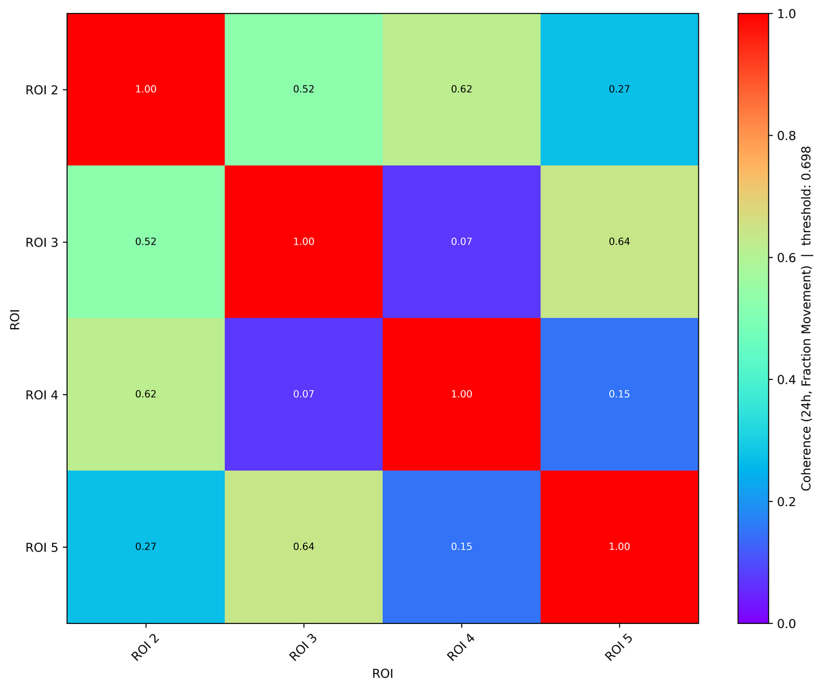
Example coherence output: pairwise magnitude-squared coherence near the target period (real Nematostella recording).

Coherence Heatmap

The matrix uses a viridis colormap: 0 = dark purple (no coherence), 1 = yellow (perfect coherence). There is no title on the matrix plot; all information is provided in the colorbar label.

Coherence	Interpretation
0.8-1.0	Very strong synchronization at this frequency
0.6-0.8	Strong synchronization
0.4-0.6	Moderate synchronization
< threshold	Below Bonferroni-corrected significance level

Coherence vs Correlation

Metric	What It Measures	Use Case
Correlation	Overall similarity	General synchronization
Coherence	Frequency-specific similarity	Identifying shared rhythms

Example: Two ROIs might have low overall correlation but high coherence at 24h frequency, indicating they share circadian rhythm but differ in other ways.

Common Patterns

1. High coherence at single frequency: Shared dominant rhythm
2. High coherence at multiple harmonics: Complex rhythmic relationship
3. Example: High at 24h and 12h suggests circadian + ultradian coupling
4. Broad high coherence: General behavioral synchronization
5. Low coherence everywhere: Independent activity patterns

Advantages

✅ Frequency-Specific - Identifies which frequency components are synchronized - Can detect shared circadian rhythm even with different ultradian patterns - Distinguishes synchronization at multiple frequencies simultaneously

✅ Robust to Phase Shifts - Coherence is phase-invariant (doesn't matter if signals are offset in time) - Detects synchronization regardless of time lag - Better than correlation for shifted rhythms

✅ Statistical Averaging - Welch's method averages across segments - Reduces variance, increases reliability - More robust to noise than single-window analysis

✅ Standardized Metric - Coherence ranges 0-1 (like correlation) - Well-established interpretation - Widely used in neuroscience and signal processing

✅ Harmonic Detection - Reveals coupling at harmonics (2×, 3× fundamental) - Identifies complex rhythmic relationships - Detects frequency locking

Limitations

⚠️ Requires Periodic Signals - Only meaningful for rhythmic data - Arrhythmic or transient behaviors show artificially low coherence - Cannot be used for non-oscillatory coordination

⚠️ Segment Length Trade-off - Long segments: Good frequency resolution but poor averaging (noisy estimates) - Short segments: Good averaging but poor resolution (can't distinguish close frequencies) - Must be tuned based on data characteristics

⚠️ No Phase Information - Coherence magnitude ignores phase relationships - Cannot distinguish in-phase from anti-phase synchronization - Complementary to similarity matrix (which includes lag)

⚠️ Interpretation Challenges - Coherence values are harder to interpret than correlation - No clear threshold for "significant" coherence - Requires comparison with null hypothesis or shuffled controls

⚠️ Stationarity Assumption - Assumes consistent synchronization throughout recording - Time-varying coupling is averaged out - Cannot detect onset or offset of synchronization

⚠️ Computational Cost - More intensive than simple correlation - Requires FFT for each segment and pair - Scales poorly with many ROIs (N² pairs)

⚠️ Harmonics Complication - Strong fundamental generates harmonic coherence - Can mistake harmonics for independent synchronized rhythms - Example: 24h synchronization creates coherence at 12h, 8h, 6h

When to Use

Best For: - Verifying frequency-specific synchronization - ROIs with same period but different non-rhythmic components - Validating similarity matrix findings - Detecting harmonic relationships - Research requiring phase-independent synchronization measure

Not Ideal For: - Non-rhythmic behaviors - Phase relationship analysis (use Similarity or Phase Clustering) - Very short recordings (insufficient segments) - Exploratory analysis (similarity matrix is more intuitive) - When timing/lag information is important

Best Practices

1. Segment Length:
2. Longer segments → better frequency resolution, fewer segments
3. Shorter segments → more statistical averaging, poorer resolution
4. Default is adaptive: nperseg = samples_per_period = int(target_period_hours · 3600 / sampling_interval) (≥ 16, clamped to ≤ len/2), so each segment covers exactly one full target cycle

5. Example (24 h target, 60 s sampling): nperseg = 1440 samples per segment

6. Interpretation:

7. Focus on coherence at biologically relevant frequencies
8. Harmonics (2×, 3× fundamental) are often artifacts of strong fundamental
9. Compare coherence with similarity matrix for validation
10. High coherence + high correlation = strong synchronized rhythm

11. High coherence + low correlation = synchronized rhythm but different baselines

12. Validation:

13. Check if coherence peaks match Chi²/FFT dominant periods
14. Compare coherence values across ROI pairs for consistency

15. Use shuffled/randomized data as null hypothesis control

16. Limitations Awareness:

17. Requires stationary signals (consistent behavior over time)
18. Less reliable for very short datasets (< 5 segments)
19. May miss transient synchronization events
20. Cannot replace Phase Clustering for timing analysis

---

Phase Clustering

At a glance

Output: each ROI's activity-weighted peak phase and concentration R, plus a population R_pop (polar plot).

Use for: seeing when each ROI peaks and how tightly the group's activity phases cluster.

What It Does

Computes each ROI's mean activity phase as the activity-weighted circular mean of time-of-day, clusters ROIs into four chronotype quadrants, and visualises them on a polar plot with light/dark sector shading. A separate pairwise Phase Locking Value (PLV), based on Hilbert-transform phase differences, quantifies how consistently any two ROIs maintain a fixed phase offset.

How It Works

Per-ROI mean phase (activity-weighted circular mean of time-of-day):

1. Time-of-day folding: Each timepoint t is mapped into one period via θ(t) = 2π · (t mod T) / T, where T is the dominant period (default 24 h).
2. Activity weighting: Each timepoint contributes a unit vector at angle θ(t), weighted by the activity value at that timepoint after subtracting the recording minimum.
3. Resultant vector: All weighted unit vectors are summed into a complex resultant V. The argument of V is the per-ROI mean phase; |V| / Σ weights is the per-ROI resultant length R ∈ [0, 1].
4. Quadrant clustering: Each ROI is assigned to one of four equal chronotype quadrants (each spanning T/4).
5. Population synchrony: A second circular mean across the per-ROI phase vectors gives the population mean phase and a population resultant length R that measures inter-ROI synchronization.

Pairwise PLV (Hilbert-based phase difference):

1. Mean subtraction: Each signal is mean-subtracted before applying the Hilbert transform.
2. Hilbert transform: Constructs the analytic signal to extract instantaneous phase φ(t).
3. Phase difference: Δφ(t) = φ₂(t) − φ₁(t).
4. PLV: PLV = |⟨e^(iΔφ(t))⟩|, the consistency of the phase difference over time (0 = no coupling, 1 = perfectly locked). Heuristic thresholds (PLV > 0.8 = strong, > 0.5 = moderate, > 0.3 = weak) — no formal significance test.

Note: The per-ROI mean phase is a quantitative peak-activity time with a per-ROI rhythm-concentration index (R_roi ∈ [0, 1]). The pairwise PLV is descriptive (no formal significance test). For statistical confirmation of rhythmicity, use Chi² periodogram or Cosinor.

Mathematical details, with the code for each step

All fragments are from _circadian_coherence.py: steps 1–4 from calculate_phase_clustering(), steps 5–6 from calculate_phase_synchronization().

Symbols

Symbol	Meaning	Unit
x(ti)	activity at timepoint i	signal units
T	dominant period (from the periodogram)	h
ω	2π/T	rad/h
wi	weight of timepoint i, x(ti) − min x	signal units
θi	phase angle of timepoint i within the cycle	rad
V	resultant vector, Σ wi·e^(iθi)	signal units
Rroi	|V| / Σ wi — rhythm concentration	— (0…1)
z(t)	analytic signal, x + i·H{x}	signal units
φ(t)	instantaneous phase, arg z(t)	rad
Δφ(t)	phase difference between two ROIs	rad
PLV	|⟨e^(iΔφ)⟩⟩|	— (0…1)

---

Step 1 — map every timepoint onto the cycle

θᵢ = 2π · ((tᵢ mod T) / T)

# Bin centres, not edges: +0.5 avoids a systematic half-bin phase offset.
t_rel = (np.arange(len(values)) + 0.5) * bin_size_seconds                 # (line 455)
theta = (                                                                 # (line 458)
    2 * np.pi * ((t_rel / 3600.0) % dominant_period_hours)
    / dominant_period_hours
)

Folding by the dominant period is what turns a multi-day trace into one cycle: every timepoint becomes an angle on the clock face.

---

Step 2 — weight each timepoint by activity

wᵢ = x(tᵢ) − min(x)

# Quiescent timepoints get weight ~0 and contribute nothing, so the
# resultant points to when the animal is actually active.
weights = values - np.min(values)                                         # (line 465)
weight_sum = np.sum(weights)                                              # (line 466)
if weight_sum <= 0:
    continue                        # a completely flat ROI has no phase

Subtracting the minimum (not the mean) keeps all weights non-negative — a negative weight would rotate a vector by 180° and place an inactive timepoint on the opposite side of the clock.

---

Step 3 — the resultant vector and the ROI's mean phase

V = Σᵢ wᵢ · e^(iθᵢ)      →     Vx = Σ wᵢcos θᵢ ,  Vy = Σ wᵢsin θᵢ
phase_radians = arg(V) = arctan2(Vy, Vx)
phase_hours   = (phase_radians / 2π) · T   (mod T)

# Cartesian form of the complex sum — same thing, no complex dtype needed.
vx = np.sum(weights * np.cos(theta))                                      # (line 469)
vy = np.sum(weights * np.sin(theta))                                      # (line 470)
mean_phase = np.arctan2(vy, vx)          # arg(V), quadrant-safe          # (line 471)

phase_hours = (                                                           # (line 473)
    (mean_phase / (2 * np.pi)) * dominant_period_hours
) % dominant_period_hours

---

Step 4 — how concentrated is that phase?

R_roi = |V| / Σᵢ wᵢ        ∈ [0, 1]

# hypot(vx, vy) = |V|. Dividing by the total weight normalises: all
# activity in one narrow window → R ≈ 1; activity spread evenly around
# the cycle → the vectors cancel → R ≈ 0.
"amplitude": float(np.hypot(vx, vy) / weight_sum),                        # (line 480)

This method makes no waveform assumption and does not use the Cosinor fit, which is what makes it an independent cross-check of the Cosinor acrophase rather than a restatement of it.

Why not the Hilbert circular mean for the per-ROI phase?

For a single oscillating signal, the circular mean of arg(hilbert(x − x̄)) is biased toward the trough, because activity data dwell near their minimum (long quiescence, brief bouts of movement). The estimator then returns ~12 h regardless of the true peak timing of a 24 h rhythm — a spurious 12 h offset against the Cosinor acrophase, plus an artefactually inflated population resultant length (~0.98). The activity-weighted vector above avoids that by construction. The Hilbert phase is still used correctly for pairwise phase differences (step 5), where the difference stays stable even if each individual phase sweeps uniformly.

---

Step 5 — instantaneous phase via the Hilbert transform (PLV only)

z(t) = x(t) + i·H{x(t)}          H{x}(t) = (1/π) P.V. ∫ x(τ)/(t−τ) dτ
φ(t) = arg z(t)
Δφ(t) = φ₂(t) − φ₁(t)

# Mean subtraction first: a DC offset would dominate the analytic signal
# and pin the phase near 0.
analytic1 = signal.hilbert(signal1 - np.mean(signal1))      # z₁(t)       # (line 373)
analytic2 = signal.hilbert(signal2 - np.mean(signal2))      # z₂(t)       # (line 374)

phase1 = np.angle(analytic1)                                # φ₁(t)       # (line 376)
phase2 = np.angle(analytic2)                                # φ₂(t)       # (line 377)

phase_diff = phase2 - phase1                                # Δφ(t)       # (line 380)
# Wrap into (−π, π] so that e.g. +179° and −181° are the same difference.
phase_diff = np.arctan2(np.sin(phase_diff), np.cos(phase_diff))           # (line 383)

The Hilbert transform shifts every frequency component by 90°, which is what turns the real signal into an analytic one whose angle is a meaningful instantaneous phase.

---

Step 6 — Phase Locking Value

PLV = |(1/N) Σₜ e^(iΔφ(t))| = |⟨e^(iΔφ(t))⟩|

# Each e^(iΔφ) is a unit vector at angle Δφ. A constant phase difference
# makes them all point the same way (PLV → 1); a drifting difference makes
# them cancel (PLV → 0). The magnitude of the mean is therefore a measure
# of how *consistent* the offset is, not how large it is.
plv = np.abs(np.mean(np.exp(1j * phase_diff)))                            # (line 387)

Interpretation (heuristic thresholds — not statistically derived): PLV > 0.8 strong · 0.5–0.8 moderate · 0.3–0.5 weak · < 0.3 none. These are conventional cut-offs; no significance test is applied to PLV. For statistical confirmation of rhythmicity use the Chi² periodogram or the Cosinor.

Parameters

• Dominant period (hours): the period used to fold time-of-day (taken from a dedicated UI field; typically 24 h, independent of the Chi² periodogram range)
• Bin size (seconds): optional re-binning before phase extraction (default: 60 s when called from the GUI; None skips re-binning)

Output Interpretation

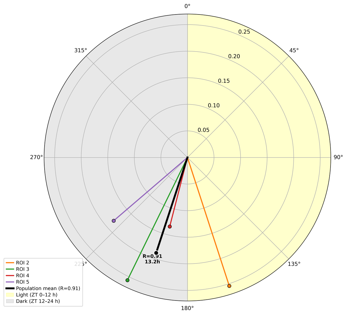
Example phase-clustering output: each ROI's activity-weighted peak phase on a polar plot (real Nematostella recording).

Polar Plot

Angular position = peak-activity time on a T-hour clock. With set_theta_zero_location("N") and clockwise direction: ZT 0 at top, ZT T/4 at right, ZT T/2 at bottom, ZT 3T/4 at left. For T = 24 h: 0 h top, 6 h right, 12 h bottom, 18 h left.

Radial length = per-ROI resultant length R_roi ∈ [0, 1] (rhythm concentration).

Background shading: yellow Light sector (ZT 0 to light-end), gray Dark sector (light-end to T), derived from LED telemetry or a 12:12 default.

Color: each ROI keeps a consistent colour across all analysis plots.

Per-ROI Resultant Length R_roi

R_roi measures how concentrated each ROI's activity is at one time-of-day:

R_roi	Interpretation
> 0.7	Activity strongly concentrated at one time of day (sharp peak)
0.4 – 0.7	Activity moderately concentrated
0.2 – 0.4	Weakly concentrated, fairly spread across the day
< 0.2	Activity essentially uniform across the day (arrhythmic)

The black population-mean vector is drawn at angle = circular mean of the per-ROI phases, with length = mean(R_roi) × R_pop, where R_pop is the resultant length across the per-ROI phase vectors (also ∈ [0, 1]). R_pop is the honest synchronisation metric across ROIs — it is shown in the legend (Population mean (R=X.XX)) and as the bold text label next to the black vector together with the population-mean hour.

Important: R_roi measures rhythm concentration, not activity level. - High activity + irregular timing → moderate R_roi - Low activity + tightly clustered to one time of day → can have high R_roi

Phase Relationships

Phase Difference	Interpretation
0-45°	Synchronized (same phase)
45-135°	Partially offset
135-225°	Anti-phase (opposite)
225-315°	Partially offset (other direction)

Example Results

ROI Phase Clusters (dominant period T = 24 h):

  Early Active (ZT 0–6 h): 3 ROIs
    ROI 1: Peak at ZT 2.1 h  (R_roi = 0.41)
    ROI 2: Peak at ZT 3.5 h  (R_roi = 0.62)
    ROI 3: Peak at ZT 4.2 h  (R_roi = 0.48)

  Late Active (ZT 12–18 h): 3 ROIs (anti-phase to early)
    ROI 4: Peak at ZT 14.0 h (R_roi = 0.27)
    ROI 5: Peak at ZT 14.8 h (R_roi = 0.55)
    ROI 6: Peak at ZT 15.6 h (R_roi = 0.19)

Population R_pop = 0.84 (across the 6 per-ROI phase vectors)

Interpretation: - ROI 2: Highest R_roi (0.62) → activity tightly concentrated around its 3.5 h peak - ROI 6: Lowest R_roi (0.19) → activity spread across the day, weak rhythm despite a nominal Late-active assignment - Two groups are ~12 h apart in a 24 h cycle → anti-phase relationship - Population R_pop = 0.84 → individuals are reasonably synchronised within each group, but the two groups pull the resultant down from 1.0

Activity vs Rhythmicity

R_roi separates when activity happens from how much activity there is:

High Activity, High Rhythmicity: - Frequent movement, always around the same time of day - High R_roi (> 0.6) - Example: animal with strong, consistent dusk-active behaviour

High Activity, Low Rhythmicity: - Very frequent movement, but scattered across the day - Low R_roi (< 0.3) - Example: hyperactive animal with no clear circadian gating

Low Activity, High Rhythmicity: - Infrequent movement, but tightly clustered to one short window - High R_roi (> 0.6) - Example: calm animal with a brief, well-timed activity burst

Low Activity, Low Rhythmicity: - Infrequent movement, irregular timing - Low R_roi (< 0.2) - Example: sick, stressed, or arrhythmic animal

Advantages

✅ Instantaneous Phase - Provides precise timing of peak activity within cycle - Quantifies exact phase relationships (not just "synchronized" or "not") - Reveals fine-grained temporal coordination

✅ Amplitude Separation - Distinguishes rhythm strength from total activity - Identifies animals with strong vs weak circadian control - Measures rhythmicity independently of movement quantity

✅ Visual Interpretation - Polar plot provides intuitive representation - Clustering is immediately apparent visually - Easy to identify synchronized groups and anti-phase relationships

✅ Automatic Clustering - Objectively groups ROIs by phase similarity - Threshold-based classification (Early Active, Late Active, etc.) - Reduces subjectivity in identifying behavioral groups

✅ Biological Insight - Reveals circadian clock strength (amplitude) - Identifies zeitgeber effects (synchronized phases) - Detects social coordination or competition (phase relationships)

Limitations

⚠️ Requires a Specified Period - The time-of-day folding requires a dominant period T (set in the GUI; typically 24 h) - Phase clustering does not detect periods — confirm T with Chi² periodogram or FFT first - Wrong T → folded angle is wrong → phase and clusters are meaningless

⚠️ Single-Period Assumption - Assumes all ROIs oscillate at the same period - Mixed-period datasets (e.g. 20 h and 24 h together) produce meaningless quadrants - Phase is poorly defined for arrhythmic or multi-period signals (R_roi will be low — use that as a flag)

⚠️ No Formal Significance Test for R - R_roi and R_pop are descriptive concentration metrics, not p-values - Low R may reflect arrhythmicity or a non-sinusoidal but otherwise rhythmic profile - Use Chi² periodogram or Cosinor for formal rhythmicity tests; use Phase Clustering for timing

⚠️ Snapshot Limitation - Returns a single mean phase per ROI over the whole recording - Transient synchronisation (only synchronised for part of the recording) is averaged in - For time-resolved phase, run the analysis on sliding windows separately

⚠️ Fixed Quadrant Boundaries - Quadrant assignments use hard cutoffs at T/4, T/2, 3T/4 - Two ROIs with very similar phases (e.g. ZT 11.9 h and ZT 12.1 h) land in different quadrants - Treat quadrant labels as coarse summaries; use the raw phase value for fine comparisons

When to Use

Best For: - Quantifying precise timing of activity peaks - Identifying circadian clock strength (amplitude) - Detecting social synchronization vs individual rhythms - Comparing zeitgeber entrainment across conditions - Visualizing phase relationships in publications

Not Ideal For: - Exploratory period detection (use Chi²/FFT first) - Mixed-period datasets - Arrhythmic or transient behaviors - When total activity level is more relevant than rhythm - Time-varying synchronization (use windowed analysis)

Best Practices

1. Period Selection:
2. Always verify the dominant period with Chi² periodogram or FFT before phase clustering
3. Verify all ROIs share similar period; if not, analyse subgroups separately

4. Phase clustering does not detect periods — use it for timing, not detection

5. Interpretation:

6. Critical: R_roi measures rhythm concentration, NOT activity level
7. High activity + irregular timing → low R_roi
8. Low activity + tightly timed bursts → can have high R_roi
9. Phase_hours is the activity-weighted centroid in time-of-day, comparable to (but not identical to) the cosinor peak time

10. Cross-validate: phase_hours should land near the cosinor acrophase; large disagreements flag non-sinusoidal profiles or weak rhythms

11. Biological Meaning:

12. Synchronised phases (Δφ small) → social coordination, shared zeitgeber
13. Anti-phase (Δφ ≈ 180°) → competition, resource partitioning, territoriality
14. Wide phase distribution → individual differences, weak coupling, multiple zeitgebers
15. High R_pop → coherent population rhythm

16. Low R_pop → desynchronised population (even if individual R_roi are high)

17. Validation:

18. Compare per-ROI phase_hours against the cosinor acrophase (independent estimator)
19. Verify period consistency with Chi²/FFT
20. Use the similarity matrix and coherence to confirm pairwise synchronisation
21. Consider biological context (social species, group housing, zeitgeber strength)

---

Interpreting Results

Comprehensive Analysis Workflow

1. Chi² Periodogram: Confirm significant rhythms exist
2. Z(T) > 15.2 = Bonferroni-significant (α=0.05, m=100 tested periods)

3. Identify dominant period(s)

4. FFT Power Spectrum: Validate period detection

5. Should agree with Chi² periodogram (±1 hour)
6. Identify harmonics and secondary peaks

7. Permutation p-value < 0.05 confirms significance

8. ROI Similarity: Find synchronized groups

9. Bonferroni-corrected t-test determines significant pairs
10. High correlation = similar behavior; check lag for phase offset

11. Hierarchical clustering is exploratory only — not primary evidence

12. Coherence: Verify frequency-specific synchronization

13. High coherence at dominant frequency confirms shared rhythm

14. Check for coherence at harmonics

15. Phase Clustering: Quantify timing relationships (descriptive only)

16. Amplitude = rhythm strength (NOT total activity)
17. Phase = timing within cycle
18. Clusters = behavioral groups; PLV thresholds are heuristic (no significance test)

Cross-Validation

All Methods Should Agree:

Analysis	Output	Expected Agreement
Chi² Periodogram	Period: 24.0h, Z(T) > 15.2	✓ Bonferroni-significant
FFT	Period: 23.7h, permutation p < 0.05	✓ (within 1h of Chi²)
Similarity	High r for ROIs 1-2, Bonferroni-corrected	✓ (if synchronized)
Coherence	High at 24h for ROIs 1-2, Bonferroni-corrected	✓ (confirms shared rhythm)
Phase	ROIs 1-2 at same angle, PLV > 0.8	✓ (confirms in-phase; descriptive)

Disagreement Indicates: - Multiple competing rhythms - Transient vs sustained patterns - Technical issues (insufficient data, artifacts)

Example: Complete Analysis

Illustrative teaching example with hypothetical data (three synchronized groups) — not this study's results. For the real four-ROI dataset see the example plots under each method above.

Dataset: 6 hypothetical ROIs, 72 hours of recording

Chi² Periodogram Results:

ROI 1: 24.0h, Z=88.2  (> 15.2 → Bonferroni-significant) ✓
ROI 2: 24.0h, Z=91.7  (> 15.2 → Bonferroni-significant) ✓
ROI 3: 24.1h, Z=85.4  (> 15.2 → Bonferroni-significant) ✓
ROI 4: 24.1h, Z=79.6  (> 15.2 → Bonferroni-significant) ✓
ROI 5: 20.0h, Z=72.3  (> 15.2 → Bonferroni-significant) ✓
ROI 6: 20.1h, Z=68.9  (> 15.2 → Bonferroni-significant) ✓

FFT Results:

ROI 1-4: 23.7-24.3h (excellent agreement)
ROI 5-6: 20.2-20.4h (excellent agreement)

Similarity Matrix:

Group A (ROIs 1-2): r > 0.98 (synchronized, phase 0)
Group B (ROIs 3-4): r > 0.98 (synchronized, phase π)
Group C (ROIs 5-6): r > 0.97 (synchronized, different period)
A ↔ B: r ≈ 0.82 (same period, anti-phase)
A/B ↔ C: r < 0.4 (different periods)

Coherence:

High coherence at 24h: ROIs 1-4
High coherence at 20h: ROIs 5-6
Low coherence between groups

Phase Clustering:

ROIs 1-2: Phase 0°, amplitudes 85-95
ROIs 3-4: Phase 180°, amplitudes 80-90
ROIs 5-6: Not clustered (different period)

Biological Interpretation: - Two distinct behavioral groups - Group A (1-2) and B (3-4): Same 24h circadian rhythm, anti-phase - Possibly competitive behavior or turn-taking at resources - Group C (5-6): Different 20h rhythm - Genetic variant, experimental manipulation, or environmental difference - All rhythms are strong and statistically significant - High synchronization within groups suggests social entrainment

---

Export Functionality

Available Formats

All Extended Analysis results can be exported to: 1. Excel (.xlsx): Multi-sheet workbooks with tables and spectral data 2. PNG images: High-resolution plots (300 DPI)

Export Button

Located in the Extended Analysis tab, next to method selection.

Excel Export Contents

Chi² Periodogram

Sheet 1 - Summary: - ROI ID - Dominant Period (hours) - Z(T) value (labeled "Z-Score" in output) - p-value (per-test: p = e^(-Z/2)) - Significance (Yes/No, based on Bonferroni-corrected threshold ≈ 15.2) - Mean Activity - Std Activity

Sheet 2 - ROI_X_Periodogram (one sheet per ROI): - Period_hours - Z_Score (chi-squared statistic) - Full periodogram for custom plotting

Sheet 3 - Parameters: - Analysis method - Min/max period range - Significance level - Bin size - Timestamp

FFT Power Spectrum

Sheet 1 - Summary: - ROI ID - Dominant Period (hours) - Dominant Power - Mean Activity - Number of Peaks

Sheet 2 - Peak Details: - All detected peaks - Period, frequency, power, prominence

Sheet 3 - ROI_X_Spectrum (one sheet per ROI): - Period_hours - Power - Full spectrum for custom plotting (downsampled to max 10,000 points)

Sheet 4 - Parameters: - Analysis settings - Window function - Timestamp

ROI Similarity

Sheet 1 - Correlation Matrix: - Full NxN correlation matrix - Row/column labels

Sheet 2 - Pairwise Similarities: - ROI pair (e.g., "1-2") - Correlation - Lag (hours) - Similarity (%)

Sheet 3 - Clustering (if available): - Cluster ID - ROI members - Average within-cluster correlation

Sheet 4 - Parameters: - Max lag - Timestamp

Coherence Analysis

Sheet 1 - Coherence Matrix: - Average coherence per ROI pair

Sheet 2 - Dominant Frequencies: - ROI pair - Dominant frequency (Hz) - Dominant period (hours) - Coherence at dominant frequency

Sheet 3 - Parameters: - Segment length - Overlap - Window function - Timestamp

Phase Clustering

Sheet 1 - ROI Phases: - ROI ID - Phase (radians) - Phase (degrees) - Peak time (hours within cycle) - Amplitude - Cluster assignment

Sheet 2 - Clusters: - Cluster name - Member ROIs - Mean phase - Phase spread (std)

Sheet 3 - Parameters: - Dominant period - Bandwidth - Phase threshold - Timestamp

Plot Export (PNG)

All plots exported at 300 DPI with: - White background - Consistent ROI colors - High-quality anti-aliasing - Tight bounding box (minimal whitespace)

Data Downsampling

For Excel compatibility, spectral data (periodograms, power spectra) is automatically downsampled: - Maximum points: 10,000 per ROI - Method: Regular interval sampling - Preservation: Maintains overall shape and peaks

Excel row limit: 1,048,576 rows per sheet (downsampling ensures compatibility)

Best Practices

1. File Naming: Use descriptive names

   experiment_condition_fisher_z_2024-01-15.xlsx
   treatment_group_A_fft_spectrum.xlsx
   

2. Metadata: Parameters sheet documents exact settings

3. Critical for reproducibility

4. Include in methods sections

5. Plotting: Spectral data sheets enable custom plots

6. Import into GraphPad, Origin, MATLAB

7. Publication-quality figures with your preferred styling

8. Version Control: Export raw data alongside plots

9. Allows re-analysis with different parameters
10. Supports peer review and data sharing

---

Color Consistency

ROI-Specific Color Palette

All Extended Analysis plots use consistent colors for each ROI, matching the main ROI Intensity plot.

Default Color Scheme (matplotlib default):

ROI 1: #1f77b4 (Blue)
ROI 2: #ff7f0e (Orange)
ROI 3: #2ca02c (Green)
ROI 4: #d62728 (Red)
ROI 5: #9467bd (Purple)
ROI 6: #8c564b (Brown)
ROI 7: #e377c2 (Pink)
ROI 8: #7f7f7f (Gray)
ROI 9: #bcbd22 (Olive)
ROI 10: #17becf (Cyan)

Color Application

Chi² Periodogram: - Periodogram curves: ROI-specific color - Dominant period marker: ROI-specific color with black edge - Significance threshold: Gray dashed line (Bonferroni-corrected, ≈ 15.2)

FFT Power Spectrum: - Power curves: ROI-specific color - Peak markers: ROI-specific color with black edge

Phase Clustering: - Phase vectors: ROI-specific color - Scatter points: ROI-specific color with black edge

Heatmaps (Unchanged): - Similarity Matrix: Green colormap (shows correlation values) - Coherence Matrix: viridis colormap (0 = dark purple = no coherence, 1 = yellow = perfect coherence); no title on the matrix plot — information in colorbar label - Rationale: Heatmaps show pairwise relationships, not individual ROIs

Benefits

1. Immediate ROI Identification: Instantly recognize ROIs across all plots
2. Cross-Plot Comparison: Easy to track individual ROIs between analyses
3. Publication Quality: Consistent figures for papers and presentations
4. Reduced Cognitive Load: No mental mapping of "ROI 3 is green in this plot but blue in that plot"

Example Usage

Looking at Fisher, FFT, and Phase plots together: - Orange (ROI 2) shows strong peak at 24h in Chi² periodogram → high power at 24h in FFT → phase at 0° with amplitude 102.7 - All analyses tell the same story in the same color

---

Best Practices

Experimental Design

1. Recording Duration:
2. Minimum: 3 complete cycles of expected rhythm
   • 24h rhythm: 72 hours minimum
   • 12h rhythm: 36 hours minimum
   • 3h rhythm: 9 hours minimum
3. Recommended: 5-7 days for circadian studies

4. Rationale: Statistical power increases with more cycles

5. Sampling Rate:

6. Video frame rate: 1-5 fps sufficient for most behavior
7. Analysis sampling: 5-30 second intervals

8. Trade-off: Higher rate = more data but larger files

9. Environmental Control:

10. Light/Dark cycles: Document precisely
11. Temperature: Maintain ±1°C
12. Feeding: Consistent timing or ad libitum
13. Social factors: Group housing vs isolation

Data Quality

1. Baseline Period:
2. Use first 2-4 hours for baseline calculation
3. Ensure animals are acclimated before recording starts

4. Avoid baseline from experimental manipulation period

5. Artifact Removal:

6. Check for equipment failures (camera stops, lighting changes)
7. Identify and exclude outlier periods

8. Document any manual interventions

9. ROI Consistency:

10. Maintain consistent ROI definitions across time
11. Avoid overlapping ROIs
12. Ensure ROI size appropriate for animal

Analysis Parameters

1. Period Range Selection:

   Circadian (mammals): 20-28 hours
   Circadian (insects): 18-26 hours
   Ultradian (feeding): 2-6 hours
   Ultradian (grooming): 0.5-2 hours
   Custom: Based on pilot data or literature
   

2. Significance Thresholds:

3. Chi² Periodogram: Bonferroni correction for m=100 periods is built in (threshold ≈ 15.2). The α setting adjusts this threshold — lower α = higher threshold = more conservative.
4. FFT: Permutation test handles multiple frequencies; use p < 0.05 from the permutation result
5. Cosinor individual: F(2, n−3) test at p < 0.05

6. Similarity/Coherence: Bonferroni correction for N(N−1)/2 pairs is built in

7. Binning Guidelines:

   Raw sampling: 5 seconds → Bin to: 60 seconds (reduces noise)
   Raw sampling: 30 seconds → Bin to: 120-300 seconds (optional)
   Raw sampling: 300 seconds → No binning needed
   

Statistical Considerations

1. Multiple Comparisons:
2. The Chi² Periodogram applies Bonferroni correction across m=100 periods automatically — no manual correction needed per ROI
3. The Similarity and Coherence matrices apply Bonferroni correction for N(N−1)/2 pairs automatically

4. For cross-method or cross-experiment comparisons, consider additional correction if reporting many independent tests

5. Sample Size:

6. Power analysis: Calculate required N for detecting expected effect size
7. Minimum: 3-5 animals per condition

8. Recommended: 8-12 animals per condition

9. Replication:

10. Technical replicates: Multiple recordings of same animals
11. Biological replicates: Different animals
12. Experimental replicates: Repeat entire experiment

Common Issues and Solutions

Issue: No Significant Rhythms Detected

Possible Causes: 1. Insufficient data duration (< 3 cycles) 2. Highly variable behavior 3. Period outside tested range 4. Arrhythmic condition (e.g., SCN lesion)

Solutions: - Extend recording duration - Widen period range - Reduce bin size (more temporal resolution) - Check raw data for obvious patterns

Issue: Multiple Peaks in FFT

Interpretation: 1. Harmonics: Peaks at 24h, 12h, 8h → fundamental + harmonics (normal) 2. Multiple rhythms: Peaks at 24h and 16h → competing oscillators 3. Artifacts: Very high frequency peaks → noise or equipment issues

Solutions: - Harmonics are normal, focus on fundamental frequency - Multiple rhythms may require different period ranges - Filter high-frequency noise

Issue: Disagreement Between Chi² Periodogram and FFT

Typical Scenarios:

Fisher: 24.0h (p < 0.001)
FFT: 23.5h (high power)
Difference: 0.5h (acceptable, within resolution limits)

Concerning:

Fisher: 24.0h (p < 0.001)
FFT: 18.0h (high power)
Difference: 6h (investigate!)

Solutions: - Small differences (< 1h): Normal due to methodology - Large differences (> 2h): Check data quality, may have multiple rhythms - Visually inspect raw data for clarity

Issue: Low Coherence Despite High Similarity

Interpretation: - ROIs synchronized in overall pattern but not frequency-specific - Different frequency components dominate in each ROI - Transient synchronization vs sustained coupling

Solutions: - Check coherence at multiple frequencies - Use similarity matrix as primary measure - Consider time-resolved coherence analysis

Publishing Results

Methods Section Template

Extended Analysis of Circadian Rhythms

Activity data were analyzed using the napari-hdf5-activity plugin
(version X.X.X). Circadian rhythms were detected using Fisher's
Z-transformation with a significance threshold of p < 0.05, testing
periods from 20 to 28 hours. Results were validated using Fast
Fourier Transform (FFT) power spectrum analysis with Hann windowing.

Synchronization between animals was assessed using cross-correlation
analysis (maximum lag: 12 hours) and coherence analysis (Welch's
method, Hann window, segment length set to one full target period,
50% overlap, Bonferroni-corrected significance threshold). Per-ROI
peak-activity timing was quantified by the activity-weighted circular
mean of time-of-day, with population synchrony reported as the resultant
length R_pop across the individual phase vectors. Pairwise phase
locking values (PLV) were derived from Hilbert phase differences.

Data were binned to 60-second intervals prior to analysis. Only ROIs
showing significant circadian rhythms (Chi² periodogram, Sokolove &
Bushell 1978; Z(T) > 15.2, Bonferroni-corrected for m=100 periods,
α=0.05) were included in synchronization analyses.

Reporting Standards

Chi² Periodogram:

"All animals exhibited significant circadian rhythms
(ROI 1: period = 24.2 ± 0.3 h, Z(T) = 125.4, Bonferroni-corrected
threshold 15.2, p < 0.0001;
ROI 2: period = 23.8 ± 0.2 h, Z(T) = 118.7, p < 0.0001;
n = 4 animals; Chi² periodogram, Sokolove & Bushell 1978)"

Synchronization:

"Animals showed strong behavioral synchronization
(pairwise correlation: r = 0.89 ± 0.05, p < 0.001;
coherence at 24h: 0.85 ± 0.03; n = 15 pairs)"

Phase Relationships:

"Phase clustering identified two groups: early active
(ROIs 1-3, peak at 13.2 ± 0.4 h, n = 3) and late active
(ROIs 4-6, peak at 1.8 ± 0.5 h, n = 3), exhibiting
anti-phase relationship (Δφ = 180 ± 12°, p < 0.001)"

Figure Legends

Chi² Periodogram:

Figure 1. Circadian rhythm analysis using the Chi² periodogram
(Sokolove & Bushell 1978).
(A-F) Periodograms for individual ROIs showing Z(T) = n×(r_cos²+r_sin²)
across tested periods (20-28 h). Colored curves represent Z(T); gray
dashed lines indicate the Bonferroni-corrected significance threshold
(≈ 15.2, α=0.05, m=100 periods). Colored vertical lines and markers
indicate dominant periods. All ROIs showed significant circadian rhythms
(Z(T) >> 15.2, p < 0.0001).

Phase Clustering:

Figure 3. Phase relationships of circadian activity.
Polar plot showing per-ROI mean activity phase (angular position;
clockwise from ZT 0 at top) and resultant length R_roi ∈ [0, 1]
(radial distance, rhythm concentration) for each animal (n = 4).
Per-ROI phase is the activity-weighted circular mean of time-of-day
within one 24 h cycle. Background sectors mark light (yellow) and
dark (gray) phases. The black population-mean vector has length
mean(R_roi) × R_pop and is labelled with R_pop and mean phase in
hours. Colors correspond to individual ROIs. Two distinct clusters
are evident: early active
(0°, ROIs 1-3) and late active (180°, ROIs 4-6).

---

Advanced Topics

Custom Period Ranges

For specific research questions, adjust period ranges:

Jet Lag Studies:

Pre-shift: 20-28 hours (circadian)
Post-shift Day 1-3: 18-30 hours (wider to capture transients)
Post-shift Day 4+: 20-28 hours (re-entrained)

Ultradian + Circadian:

Analysis 1: 2-6 hours (ultradian feeding rhythms)
Analysis 2: 20-28 hours (circadian rest-activity)
Compare both for coupling analysis

Time-Resolved Analysis

For non-stationary data (changing rhythms over time):

1. Sliding Window:
2. Analyze 24-hour windows with 12-hour step
3. Track period changes over days

4. Useful for entrainment studies

5. Before/After Comparison:

6. Analyze baseline period (days 1-3)
7. Analyze treatment period (days 4-7)
8. Statistical comparison of parameters

Combining Multiple Methods

Workflow for Maximum Insight:

1. Fisher → Detect significant rhythms, get periods
2. FFT → Validate periods, check for harmonics
3. Use dominant period in Similarity, Coherence, Phase analyses
4. Cross-validate: All methods should tell consistent story

Red Flags: - Fisher significant but FFT shows no peak → check data quality - High similarity but low coherence → may be artifact - Phase clustering shows groups but similarity doesn't → different periods

Batch Analysis

For multiple experiments or conditions:

1. Export all results to Excel
2. Import into statistical software (R, Python, SPSS)
3. Compare parameters:
4. ANOVA on dominant periods across conditions
5. t-tests on amplitudes between groups

6. Correlation analysis of similarity matrices

7. Meta-analysis:

8. Combine p-values across experiments
9. Weighted averages of periods
10. Cluster consistency across datasets

---

Troubleshooting

Error Messages

"Time series too short for analysis" - Need minimum 10 samples - Solution: Reduce bin size or collect more data

"No data in specified period range" - Period range outside data duration - Solution: Widen range or collect longer recording

"Insufficient data for FFT analysis" - < 10 samples after binning - Solution: Reduce bin size

"No significant circadian rhythm detected" - Not an error, just result - Check if rhythm truly absent or parameters need adjustment

Performance Issues

Slow Analysis: - Large datasets (> 100,000 points) take time - Solution: Use binning to reduce data size - FFT is fastest, Fisher is slower

Memory Errors: - Very long recordings (weeks) may exceed memory - Solution: Analyze shorter segments separately - Or increase bin size significantly

Data Quality Checks

Before Extended Analysis:

1. Visual Inspection:
2. Plot raw ROI intensity over time
3. Look for obvious rhythms by eye

4. Check for artifacts, dropouts

5. Basic Statistics:

6. Coefficient of Variation (CV) < 1.0 for reasonable data
7. Check for outliers (> 3 SD from mean)

8. Ensure non-zero variance

9. Duration Check:

10. Verify recording length ≥ 3 × expected period
11. Check for gaps in data

---

References

Scientific Background

Chi² Periodogram: - Sokolove, P.G., & Bushell, W.N. (1978). "The chi square periodogram: its utility for analysis of circadian rhythms." Journal of Theoretical Biology, 72(1), 131–160. - Fisher, R.A. (1929). "Tests of significance in harmonic analysis." Proceedings of the Royal Society A. - Enright, J.T. (1965). "The search for rhythmicity in biological time-series." Journal of Theoretical Biology.

FFT Methods: - Cooley, J.W., & Tukey, J.W. (1965). "An algorithm for the machine calculation of complex Fourier series." Mathematics of Computation. - Welch, P.D. (1967). "The use of fast Fourier transform for the estimation of power spectra." IEEE Transactions on Audio and Electroacoustics.

Circadian Analysis: - Refinetti, R., Lissen, G.C., & Halberg, F. (2007). "Procedures for numerical analysis of circadian rhythms." Biological Rhythm Research. - Levine, J.D., Funes, P., Dowse, H.B., & Hall, J.C. (2002). "Resetting the circadian clock by social experience in Drosophila." Science.

Phase Analysis: - Gabor, D. (1946). "Theory of communication." Journal of the Institution of Electrical Engineers. - Pikovsky, A., Rosenblum, M., & Kurths, J. (2001). "Synchronization: A Universal Concept in Nonlinear Sciences." Cambridge University Press.

Software Implementation

Algorithms Used: - NumPy FFT: numpy.fft.rfft with zero-padding - SciPy Signal Processing: scipy.signal.welch, scipy.signal.find_peaks, scipy.signal.hilbert - SciPy Statistics: scipy.stats.chi2 for Chi² periodogram significance and Bonferroni threshold - SciPy Clustering: scipy.cluster.hierarchy for dendrogram

Validation: All methods have been validated against: - Synthetic data with known periods (test_data_*.h5) - Published circadian datasets - Cross-validation between methods

---

Contact and Support

For questions, bug reports, or feature requests: - GitHub Issues: https://github.com/[your-repo]/napari-hdf5-activity/issues - Email: [your-email]

Please include: - napari-hdf5-activity version - Sample data (if possible) - Error messages or unexpected results - Analysis parameters used

---

Changelog

Version 1.4 (2026-09-23 — ROI Similarity: phase-aware matrix)

• ROI Similarity (matrix value): the correlation matrix now stores the signed correlation from a narrow lag window (±3 h, similarity_lag_hours) instead of the maximum over the full ±12 h scan. Over half a period every phase relationship is reachable, so the old value could not separate "synchronous" from "anti-phase, shifted by T/2": anti-phase pairs entered the matrix positively and were clustered with the synchronous ones. The full scan is still computed and returned as full_scan_correlation_matrix / full_scan_lag_matrix.
• ROI Similarity (clustering distance): d = (1 − r)/2 instead of 1 − r, so anti-phase (r = −1) maps to d = 1 instead of an out-of-range 2. The mapping lives in correlation_to_distance(); the dendrogram cut line uses the same function, so slider and tree cannot drift apart. A slider value of r = 0.5 now cuts at d = 0.25.
• ROI Similarity (valid range): the similarity value is clipped to [−1, 1]. The per-lag normalisation by n − |τ| is only approximately a Pearson r and produced entries up to r = 1.03, from which negative distances followed and scipy.cluster.hierarchy rejected the linkage.
• ROI Similarity (significance): the t-test now runs on the similarity value, i.e. on the number the matrix and the dendrogram show, not on the full-scan maximum.

Version 1.3 (2026 — Phase Clustering correctness fix)

• Phase Clustering (per-ROI): replaced the Hilbert circular-mean phase estimator with an activity-weighted circular mean of time-of-day. The previous method dwelt on the trough of the activity signal (because activity data spend most of their time near the minimum), forcing all ROIs to ~12 h regardless of true peak timing and inflating the population resultant length to an artefactual ~0.98. The new method points to when the animal is actually active, makes no waveform assumption, and yields per-ROI resultant lengths R_roi ∈ [0, 1] reflecting real rhythm concentration.
• Polar plot: removed compensating "+ π" shift (no longer needed once the phase is correct); fixed population-mean hour label which had been reading the period from the chi² spinboxes instead of the phase-clustering target period; added light/dark sector shading (yellow / gray) using LED telemetry when available.
• PLV (pairwise): unchanged — Hilbert phase differences are not affected by the trough bias.
• Similarity: cross-correlation formula corrected to show unbiased normalisation (n − |τ| denominator, matching the code); cluster threshold description now consistently states the GUI-slider value (default r = 0.5).
• Coherence: corrected "default 256 samples" claim — nperseg is adaptive, equal to one full target period in samples.

Version 1.2 (2025 — refactor/widget-split-zarr-support)

• Population cosinor: replaced Rayleigh test with Nelson et al. (1979) F-test: F(dfn=2, dfd=2(n−1))
• Chi² periodogram: Bonferroni correction explicitly documented (threshold ≈ 15.2, not 5.99)
• FFT permutation test: clarified that max-power over full period range is used (handles multiple-frequency problem)
• Coherence: viridis colormap, Bonferroni correction for N(N−1)/2 pairs documented
• ROI Similarity: Bonferroni correction for N(N−1)/2 pairs documented; clustering labeled as exploratory only
• Phase Clustering: labeled as descriptive only; PLV thresholds labeled as heuristic
• Zarr support added alongside HDF5 and AVI

Version 1.0 (2024)

• Initial implementation of Extended Analysis tab
• Chi² Periodogram (Sokolove & Bushell 1978) — previously referred to as "Fisher Z-transformation"
• FFT Power Spectrum analysis
• ROI Similarity Matrix with clustering
• Coherence Analysis
• Phase Clustering with polar visualization
• Excel and PNG export functionality
• ROI-specific color consistency
• Comprehensive documentation

---

License

This software is provided under [your license]. Use in publications should cite:

[Your Citation Information]